A Nonstationary Mathematical Model for Acceleration Time Series

Introduction

Both time and frequency domains are utilized to generate acceleration time series from stochastic models. Extensive reviews of acceleration time series process models in the frequency and times domain have been presented by[1], [2], and [3]. A number of papers in the literature have reported ARMA models. ARMA models are discussed in detail by Box and Jenkins [4]. The basic concept of using artificial acceleration in the seismic analysis was proposed by [5], [6], and other researchers have studied the correlation between model parameters [7], [8].

Arma Models

The autoregressive moving average ARMA models at any time step “k” may be represented as follows:

where φ1, θ1 are constant coefficients.

The eq. 1’s left side represents the autoregressive, AR, part of the order “p.” Thus, the measured data sequence used is time series []. Meanwhile, the eq. 1’s right side as part of order “q” is the moving average, MA. Then, the sequence [] is a set of identically distributed and independent Gaussian variables.

It must be said that the digitized data  is first normalized in this study. Estimating the variance or modulating function is a critical problem in modeling acceleration time series since it controls the nonstationarity of the process and statistical parameters, such as the extreme values of acceleration and structural response. The root mean square of  is calculated for a moving window of hundredfold steps centered on time step “t.” The given acceleration time series is then normalized to obtain a stationary acceleration time series, , with zero unit variance and mean.

Hence,  is considered as a stationary process of the eq. 1.

Referring to the pattern of the partial autocorrelation and autocorrelation functions is a necessary step to clarify information about the ARMA process’s order selection (p,q).

Estimation of the number of parameters and their numerical values to fit a model to a time series is a basic problem. The estimation of parameters is based on the nonlinear least squares, but the order of the model is based on the Akaike [8] Information criterion.

Application of Arma Models for Acceleration Time Series

Data

In this study, the data consist of three acceleration time series were measured: Afroun with 16000 data points digitized at 0.005 seconds, Ain Defla with 5000 data points digitized at 0.005 seconds, and Dar El Beida with 5528 data points digitized at 0.005 seconds. Shown in Fig. 1, Fig. 2, Fig. 3 are plots of the measured acceleration time series.

Modeling Procedure

The following five-step algorithm must be performed when installing the ARMA model in an acceleration time series:

1. Calculate the experimental modulating function  and normalize the given acceleration time series.
2. Suppose a simple general analytical form f(t) to fit the modulating function , and estimate the parameters .

Shown in Fig. 4, Fig. 5, and Fig. 6 are the modulating and envelope functions for the three measured acceleration time series.

1. Select the order (p,q) based on the partial autocorrelation and autocorrelation and functions.
2. Estimate the coefficients , i=1,2,…,p and 

Select the model order based on the AIC (p,q) criterion.

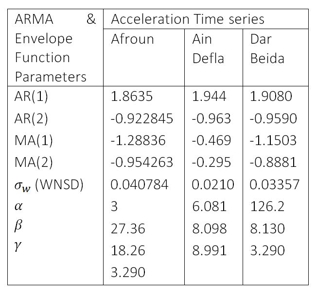
It must be said that to perform steps 3 and 4 it is necessary to apply STATGRAPHICS [9]. The ARMA parameters and envelope function parameters are shown in Table-1.

Table-1: ARMA and Envelope Function Parameters

Acceleration Time Series Simulation

To simulate acceleration time series, stationary time series are first generated using the fitted ARMA model and then multiplied by the fitted parametric envelope function eq. 3. Since ARMA model is a linear combination of past values of  and Gaussian values, simulated time series can be generated recursively.  are Gaussian random variables with zero mean and variance  . Shown in Fig. 7, 8, are simulated acceleration times series from the ARMA (2,2) models as fitted to Ain Defla, and Dar Beida Acceleration time series.

Response Spectra

The ARMA models provide an effective means in characterizing the nonstationarity of records which can be used as input in structural analysis. Each acceleration time series is an output time-series event from a representative class of stochastic processes characterized by the ARMA models.

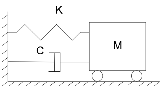
Structural response spectra provide an excellent means to describe a ground acceleration time series. A single degree of freedom system with viscous damping is used to obtain the spectral response. Fig. 9. System stiffness can be bilinear or stiffness degrading. Then, it is necessary to apply a stepwise numerical integration of the general equation that considers the linear acceleration at each time step [12]. This strategy is used to obtain the spectral response for a unique acceleration time series. The equation is:

where  is the relative mass displacement for the ground, c is the damping coefficient, M is the mass, and  is the acceleration of M is the mass relative to the fixed reference axis, and  is the restoring force.

Damage Measures

Several measures have been proposed by a number of investigators. These damage measures are expressed as functions of structural response parameters to summarize the effect of acceleration time series on linear and no-linear systems. A comparative of damage measures study was made by [10], the implementation of these arrangements has been carried out by [11].

Maximum Displacement

For design purposes, it is generally essential to know the maximum absolute value of the response subjected to an acceleration time series.

This dependence function, reflecting the relationship between the maximum value and the period or frequency of natural vibration, provides a classical spectrum for systems with the same damping value and periodic range.

Maximum Displacement Ductility

If the maximum absolute value of the displacement response calculated at its full excitation is divided by the value of the yield displacement of the system, it becomes possible to obtain the maximum displacement ductility realized as a normalized value. Thus, the maximum displacement ductility μ less than one indicates an elastic response.

Normalized Hysteretic Energy

If the amount of energy expended by the system to dissipate in the case of full excitation is divided by twice the energy absorbed at the first yield plus one, it is possible to obtain hysteretic energy, defined as the normalized value. The energy dissipated in a structure with the hysteretic load-deformation relationship is given by

where  is the elastic strain energy given by:

The normalized hysteretic energy will be then

Applications and Results

Multiple ARMA models were successfully used to analyze the three acceleration time series, with empirical data recorded for further processing. For ease of visualization, information on the projected ARMA parameters and envelope functions are summarized in Table 1. Consequently, the following steps were used to build the models. First, a sample of ten artificial acceleration time series was generated for each parameter set of the three natural series, and as illustrated in Fig. 7 and 8, even the simple model generally described well the periodicity of events peculiar to the Afroun and Dar Beida acceleration series.

Then, the damping ratio numerical values  with yield ratio  of 0.05, 0.1, 0.15, 0.2, 0.3 were used for the response analysis. Other yield ratios were used for the hysteretic energy.

Subsequently, the hysteretic energy demand spectra coupled with the mean displacement ductility were calculated for the three acceleration time series. To establish a confidence interval, the standard deviation was computed for each output event. The results are shown in Fig 9 to Fig. 20. In addition, the results were obtained using bilinear and stiffness degrading systems.

As a general remark, the spectra ordinates decrease with an increase in the period. The mean response spectra show a stable and smooth curve with changing frequencies. Spectral ordinates for both stiffness degrading systems and bilinear ones are in general similar spectral shapes.

Since the inelastic response is affected by the initial yield displacement, the yield strength ratio, which provides the initial yield displacement, is the most critical factor in the analysis of nonlinear systems.

Figs. 21, 22, 23 show typical examples of displacement ductility for yield ratios of 0.05, 0.1, 0.15, 0.2, 0.3, assuming 5% damping for a bilinear system.

Figs. 24, 25, 26 show typical examples of hysteretic energy for yield ratios of 0.01, 0.02, 0.03, 0.04, assuming 5% damping for a bilinear system.

Several useful patterns emerged from this analysis. First of all, the results obtained for the spectral response for the two quantities showed that the logarithm of the average nonlinear response demand spectrum was linearly related to the logarithm of the natural period under certain conditions. Then, based on the empirical relationships for the normalized hysteretic energy demand spectra  and for the displacement ductility μ , the following relationships can be inferred::

where , , ,  are constants related to Model and system parameters, and T natural period.

Conclusions

1. In fact, the application of the time-domain approach using ARMA models provides uncomplicated results for a limited number of parameters, while practical implementation requires imposing restrictions on the number of model parameters.
2. A good description of the average spectral response can be derived from the assumption that the acceleration time-series event is one of the sampling realizations for the set of such time series corresponding to the baseline event
3. A generally linear relationship was also found between the logarithm of the average spectra of the nonlinear response of the two quantities and the logarithm of the system’s natural period.
4. For a given system period and damping, the response spectra (displacement ductility and Hysteretic energy) decrease when the logarithm of the system period increases.

References

1. Kozin, F., 1988 “Autoregressive Moving Average Models of Earthquake records,” Probabilistic Engineering Mechanics Journal, Vol. 3, Issue 2, pp. 57-112.
2. Shinozuka, M., Deodatis, G.,and Harada, T., 1987 “Digital Simulation of Seismic Ground Motion,” Proceedings, US-Japan, Joint Seminar on Stochastic Approaches in Earthquakes, Florida Atlantic University, Boca Raton.
3. Chang, M.K., Kwiatowski, J.W., Nau, R.F., Oliver, R.M., and Pister, K.S., 1979, “ARMA models for Earthquake Ground Motion,” Rep. ORC79-1, Operation Research Center, University of California, Berkley.
4. Box, G. E. P. and Jenkins, G. M., Gregory C. R., 2008” Time Series Analysis Forecasting and Control “, Forth Edition, New Jersey, Wiley.
5. Housner, D.E., G.W., and Jennings, P.C., 1964,”Generation of Artificial Earthquakes,”Proc. ASCE, 90, No. EM1, pp.113-150.
6. Jack W. Baker, 2019 “ Conditional Mean Spectrum: Tool for Ground Motion Selection,” Journal for Structural Engineering, V. 137 Issue 3, 2011.
7. Pedersen J. and Rohde V. “Stochastic Delay Differential Equations and related Autoregressive Models,” Stochastic: An International Journal of Probability and Stochastic Processes.
8. Akaike, H. 1974, “A New Look at Statistical Model Identification IEEE Trans. Auto Contr. Vol. 19, pp. 716-723.
9. STATGRAPHICS 18, Software program, Copyright 2015 by Statpoint Technology, Inc.
10. Grigoriu, M., 1987, “Damage Models for Seismic Analysis, ”Dep. Of Civil Eng.., Cornell University.
11. Pappas, S. Sp., Ekonomou, L., Karamousantas, D., Chatzarakis, Katsikas S.,Liatsis, P, 2008 ”Electricity demand loads, modeling using Autoregressive Moving Average (ARMA) models,” Energy Journal, Vol. 33, Issue 9, pp. 1353-1360.
12. Boore, D.M. , and Atkinson, 1987, “Stochastic Prediction of Ground Motion and Spectral Response Parameters at hard-Rock Sites in Eastern North America,” Bull. Seismol. Soc. Am., pp. 440-465.
13. Chopra A.K., 2017, ’Dynamics of Structures 5^thedition,” University of California at Berkley, Pearson.