Introduction
Most statistical techniques assume that distributions of scores on dependent variables are normal. In this case, a normal distribution represents a symmetrical, bell-shaped curve, which has the greatest frequency of scores in the middle, with smaller frequencies towards the extremes (Gravetter and Wallnau, 2000; Everitt, 1996).
Skewness tests for instrument normality indicate the tilt or lack of it in distribution of respondents (Kline, 1986). These are right and left skewness whereby right skew are common. Some authors have argued that skew should have a range of +2 to -2 to indicate normal distribution. However, others statisticians apply a stringent rule of + 1 to – 1 to assess normality of instruments. In the latter case, the test for normality is critical. Positive skewness shows positive skew i.e. this is whereby scores are to the left at the low values. Conversely, negative skewness shows scores clustering at the high end. This is the right-hand side of the chart. Tabachnick and Fidell argue that when case samples are reasonable large skewness will not “make a substantive difference in analysis” (Tabachnick and Fidell, 2001).
Kurtosis indicates peaked distribution of samples. Positive Kurtosis shows clustering of samples at the center with long, thin tails. Kurtosis values below zero show relatively flat distributions i.e. there are many samples in the extremes.
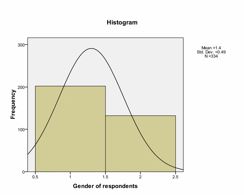
This histogram indicates that there is a positive skewness whereby most of the respondents were mainly male. The skewness is positive at 0.431 while Kurtosis is at – 1.826. According to James Dean Brown, normal distributions result into a skewness value of about zero (Brown, 1997). Thus, 0.431 value of skewness is an acceptable value of normal distribution because it is close to zero, and the difference could happen by chance. This is also within the range of + or – 2. A normal Kurtosis is usually zero. Kurtosis value of – 1.826 shows a relatively flat distribution. However, this value is within the acceptable range.
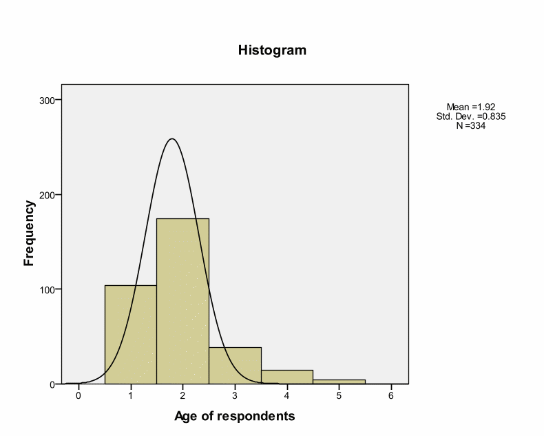
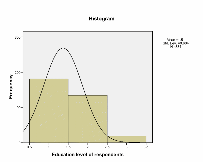
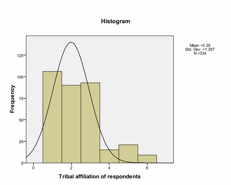
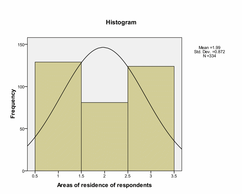
Skewness and Kurtosis values indicate that research instruments are within the acceptable ranges of – or + 2. This implies a normal distribution. However, Kolmogorov-Smirnov tests for normality indicate Significance values of.000 as shown in the below table. Kolmogorov-Smirnov test shows statistical evaluation between the practical and theoretical case of normal distribution (the significance value is.05). However, Kolmogorov-Smirnov tests for normality indicate Significance values of.000 as shown in the below table. Kolmogorov-Smirnov test shows statistical evaluation between the practical and theoretical case of normal distribution (the significance value is.05). These deviations could occur by chance because deviations are small from the recommended value. Thus, we can treat distribution as normal. Pallant argues that such cases can occur in large samples by chance (Pallant, 2005). Brown insists that skewness and Kurtosis values interpretation depend on the purpose and type of tests under analyses.
Test of reliability of the instrument
Reliability of an instrument scale should show how it is free from common errors (DeVellis, 2003; Cooper and Schindler, 2003). We can assess the reliability of a scale using test-retest reliability and internal consistency. In this case, the researcher used internal consistency to assess the reliability of research instruments. Internal consistency demonstrates the “extent to which research items that form the scale measure the same underlying attribute i.e. the extent to which the items ‘hang together” (Pallant, 2005). This research relies on Cronbach’s coefficient alpha in SPSS to measure internal consistency of instruments. This is a common method among statisticians when testing instruments reliability (Smithson, 2000). The Cronbach’s coefficient shows the average correlation among all instruments that form the scale of research. Theoretically, coefficient value for reliability ranges from 0 to 1, where higher value shows greater reliability.
Different statisticians have recommended different levels of reliability. However, these recommendations depend on the nature and use of the instrument. Nunnally proposed a lower level of 0.7 (Nunnally, 1978). It is important to note that the value of Cronbach alpha relies on the number of items on the instrument. When an instrument scale has fewer than ten items, then the Cronbach alpha values can be small. However, scale reliability also differs in terms of research samples used.
From the data, we can observe internal consistency of items of the scale as follows.
According to Nunnally, internal consistency Cronbach’s Alpha value should be 0.7. However, in this case, we have a Cronbach’s Alpha of 0.313. This value is lower than 0.7. Thus, it means that the scale items do not have internal consistency. According to Lord and Novick, SPSS may generate Alpha value that is lower than the normal range (Lord and Novick, 1968). Lord and Novick argue that Alpha “is actually a lower bound on the true reliability of a test under general conditions and that it will only equal the true reliability if items satisfy a property known as essential t – equivalence” (Lord and Novick, 1968). This suggestion requires that all items should have same values, or we can use a constant value to turn true score of every item to any other item’s true score. Thus, the implication is that the Alpha value for reliability should measure the same thing instead of a lower bound.
We must also note that reliability can range from 0.00 to 1. This suggests that Cronbach Alpha is flexible in determining perceived differences among instruments. However, reliability is not inherent in items themselves. Instead, it estimates internal consistency of various items administered to certain respondents depending on time, condition, and purpose.
Descriptive statistical test
Descriptive tests provide information about all research instruments. Descriptive tests give basic information such as mean, media, standard deviation, range, maximum, minimum, and variance. This test enables the researcher to describe characteristics of research samples, check for possibilities of violation of assumptions, and provide answers on a certain research questions. This test enables the researcher to describe characteristics of research samples, check for possibilities of violation of assumptions, and provide answers on a certain research questions (Boyce, 2003; Greene and d’Oliveira, 1999).
Inferential statistical test (Analysis of Variance)
In inferential statistical tests, the researcher attempts to reach a conclusion. Thus, the main aims of these tests are to show what the respondents think. In addition, we can use inferential statistical tests for evaluation of observed differences in dependability or occurrences by chances in study instruments (Hayes, 2000).
Analysis of Variance (ANOVA) shall tell the researcher presence of statistically significant difference between the means of three or more sets of data (Harris, 1994). In addition, the researcher can also explore the size of the difference that exists among variables. This is the Effect Size. We can determine the Effect Size through the partial eta-squared statistic (Keppel and Zedeck, 1989).
One-way ANOVA works like a t-test. However, One-way ANOVA is useful in cases where the researcher has two or more variables wants to compare the mean scores of such variables (Hair, Tatham, Anderson and Black, 1998). This test is useful when the researcher wants to determine the effect of only one independent variable on dependent variable (Stevens, 1996). However, ANOVA cannot tell where the significance difference is. Thus, the researcher can conduct post hoc comparisons to determine the significance among groups. The researcher tested if there is a difference between age groups and tribal affiliations of subjects and establish as follows.
The test of homogeneity of variances in the above case gives Levene’s test for homogeneity that illustrates whether the scores are the same for samples of the groups. The Significance value (Sig.) in this case.542. Thus, it is greater than.05. This implies that the researcher has not “violated the assumption of homogeneity of variance” (Pallant, 2005).
From the ANOVA table, the researcher has interests the significance value of Tribal affiliation of respondents. According to Pallant, “if the significance value is less than or equal to.05 (e.g..03,.01,.001), then there is a significant difference somewhere among the mean scores on your dependent variable for the groups”. In this case, the significance value is.844. This indicates that there is no significance between these pairs.
From the above data, we can present the result as follows. The researcher conducted a one-way between-groups analysis to explore the effect of age on level of tribal affiliation. The researcher grouped the respondents according to their age (Age: 18 to 25, 26 to 35, 36 to 45, 46 to 55, and 56 to 65). The researcher established that there was no statistically significance effect within the groups as the Significance was.844. This value is above the range of.05. We can also notice this value from Tukey HSD with a Significance value of.921. A number of researchers concur that they should not discuss non-significant results (Grimm and Yarnold, 1995). This is because such results indicate actual differences between groups.
Two-way ANOVA enables the researcher to test “the effect of two independent variables on one dependent variable” (Harris, 1994). From this analysis, we can see the interaction effect. This implies that we can see the influence of one independent variable on another. At the same time, we can also test the overall or main effect every independent variable.
A two-way ANOVA to show effects of gender and tribe, and education of the subjects revealed the following effects.
The Levene’s Test of Equality of Error Variances provides the researcher with the significance value of.002. This is less than.05. Thus, it is significant. Significant value suggests that the variance of dependent variable across the group is not equal. The value is less than.05. Thus, we shall consider the main effect and interaction effect among subjects. The Levene’s Test of Equality of Error Variances provides the researcher with the significance value of.002. This is less than.05. Thus, it is significant. Significant value suggests that the variance of dependent variable across the group is not equal. The value is less than.05 thus, we shall consider the main effect and interaction effect among subjects. From the Tests of Between-Subjects Effects, we have several pieces of information as follows.
The interaction effects show possibilities of any interaction effect among variables. For instance, we look at the effect of age on education levels, and whether it depends on whether the respondents are male or female.
The significance result in this table is the area marked GENDER*TRIBE. In order to determine the significance interaction, we check the significance column for the value. We consider any value that falls within the significance range of.05 (equal to or less than.05). Such values enable the researcher conclude that there is a significant interaction effect. In this case, the interaction effect is.405 (GENDER*TRIBE: Sig. =.405) this is [F (5, 333).364, p =.405)]. This value indicates the lack of significant difference in the effect of age on the level of education among female and male respondents.
Main effect
There is no significant interaction in the above case. Consequently, we can look at the main effects i.e. the effect on “a single independent variable on other variables” (Pallant, 2005). For instance, we take look at the variable GENDER so as to determine whether we have main effect for every independent variable. We check significance column for every variable. Any value than is less than or equal to.05 indicates a significant main effect for that particular variable. For GENDER, we have significance value of.286. Thus, there is no main effect. However, for TRIBE, the significance value is.009. This is less than.05. Thus, we have significant of main effect. Male and female do not differ in their levels of education. However, there is a difference among tribes in terms of their ages.
Effect size
We can locate the effect size for TRIBE on the Partial Eta Squared column. This value is.046. If we consider Cohen’s criterion, then this effect size is small (Cohen, 1988). This is statistical significance. We can see this from the Descriptive statistics of gender across all tribes (see below). The difference is little for any practical significance.
Post hoc tests
This shall help us determine where the differences exist among various tribes. This provides a systematically difference among means for all pairs of the groups. We have significant main effect for TRIBE. Thus, we can determine where differences exist using multiple comparisons.
Multiple comparisons use Tukey HSD to show significance differences among variables. In this column, we check values that are less than.05. We can also identify where the differences exist from the asterisk in the Mean Difference column (see below). We have significance difference among Luo and Kikuyu (Sig. =.029), Kalenjin and Kikuyu (Sig. =.042).
The plot shows the impact of tribe on education across.
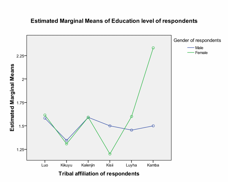
We can conclude that the two-way ANOVA between groups explored the effect of tribes on education levels among the respondents. The researcher grouped the respondents according to their tribes (Luo, Kalenjin, Kikuyu, Luyha, Kamba, and Kisii). We found significant main effect for tribes at Sig. value of.009. However, Partial Eta Squared revealed that the effect size was small (.046). Post hoc tests using the Tukey HSD scale showed that the significant difference existed among Luo, Kikuyu, and Kalenjin. The rest of the groups did not have significance differences.
References
Boyce, J. (2003). Market research in practice. Boston: McGraw-Hill.
Brown, J. D. (1997). Skewness and kurtosis. Shiken: JALT Testing & Evaluation, 1(1), 20-23.
Cohen, J. W. (1988). Statistical power analysis for the behavioral sciences (2nd ed.). Hillsdale, NJ: Lawrence Erlbaum Associates.
Cooper, D. R. and Schindler, P. S. (2003). Business research methods (8th ed.). Boston: McGraw-Hill.
DeVellis, R. F. (2003). Scale development: Theory and applications (2nd ed.). Thousand Oaks, California: Sage.
Everitt, B. S. (1996). Making sense of statistics in psychology: A second level course. Oxford: Oxford University Press.
Gravetter, F. J. and Wallnau, B. (2000). Statistics for the behavioral sciences (5th ed.). Belmont, CA: Wadsworth.
Greene, J. and d’Oliveira, M. (1999). Learning to use statistical tests in psychology (2nd ed.). Buckingham: Open University Press.
Grimm, L. G. and Yarnold, P. R. (1995). Reading and understanding multivariate statistics. Washington, DC: American Psychological Association.
Hair, J. F., Tatham, R. L., Anderson, R. E. and Black, W. C. (1998). Multivariate data analysis (5th ed.). New York: Prentice Hall.
Harris, R. J. (1994). ANOVA: An analysis of variance primer. Itasca, Ill: Peacock.
Hayes, N. (2000). Doing psychological research: Gathering and analysing data. Buckingham: Open University Press.
Keppel, G. and Zedeck, S. (1989). Data analysis for research designs: Analysis of variance and multiple regression/correlation approaches. New York: Freeman.
Kline, P. (1986). A handbook of test construction. New York: Methuen.
Lord, F. M. and Novick, M. R. (1968). Statistical theories of mental test scores. Reading, MA: Addison-Wesley.
Nunnally, J. O. (1978). Psychometric theory. New York: McGraw-Hill.
Pallant, J. (2005). SPSS Survival Manual. Sydney: Ligare.
Smithson, M. (2000). Statistics with confidence. London: Sage.
Stevens, J. (1996). Applied multivariate statistics for the social sciences (3rd ed.). Mahway, NJ: Lawrence Erlbaum.
Tabachnick, B. G. and Fidell, L. S. (2001). Using multivariate statistics (4th ed.). New York: HarperCollins.