Introduction
The purpose of this experiment is to test the relationship between an athlete’s winning percentage and the athlete’s ability to deal with pressure, focus, and their overall enjoyment of the sport. A survey was conducted by calculating 60 different athlete’s (20 high school, 20 college, and 20 pro) overall winning percentages and all athletes were made to respond to a three question survey. The questionnaire involved a Likert scale from 1(least) to 5 (most).
This report presents an analysis of the results derived from the participants’ responses. The analysis will involve an ANOVA test with post hoc Simple Linear Regression/Correlation Chi Square. The ANOVA test will identify the presence of any relationship between an athlete’s level and the 4 variables (winning percentage, pressure, focus, enjoyment). The regression/correlation analysis will investigate if there is any relationship between winning percentage and pressure, focus, or enjoyment. The strongest relationship with winning percentage will be investigated, as well as the difference in these relationships amongst the athletes.
A Chi Square test will be used to investigate the influence of an athlete’s level on the athlete’s ability to manage pressure, focus, and overall enjoyment of the sport. The analysis will be used to provide responses to the following questions:
- What is the main finding of the research study?
- Were all three statistics required to answer the study question?
- What is the benefit of using the three different statistics for the research?
Study Sample
The sample was comprised of sixty athletes. The participants were selected using a stratified random sampling method. The advantage of using this method was that it allowed the researcher to select the participants across the different athlete levels intended for the study (Bluman, 2012). The sample is different from the population in the sense that the population may comprise of both athletes and non-athletes in general (Lane, 2005). The sample focuses on athletes within three experience levels.
Results and Analysis
ANOVA Test
The ANOVA test was performed to identify the presence of any relationship between an athlete’s level and the 4 variables (winning percentage, pressure, focus, enjoyment).
Table 1: ANOVA Test Results.
Table 2: Post-hoc Results (Tukey Test).
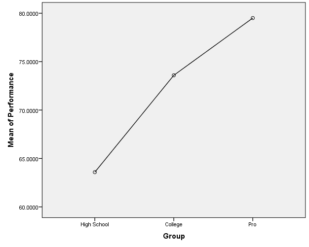
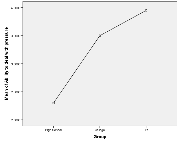
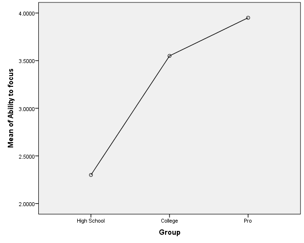
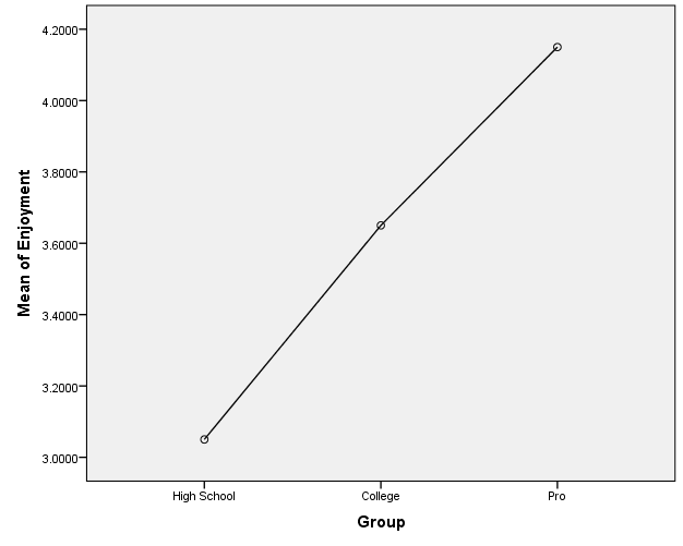
Figures 1, 2, 3, and 4 present the plots of the means for each group against the four variables. It is easy to observe from the plot pro athletes score highest for each variable mean scores, followed by college athletes, and high school athletes. The plots indicate that the group has an influence on all the variables.
Regression/ Correlation Analysis
The regression/correlation analysis investigated the relationship between winning percentage and pressure, focus, or enjoyment. The strongest relationship with winning percentage was also investigated, as well as the difference in these relationships amongst the athletes. The table below is a summary of the data collected the regression analysis. The data were used to plot three scatter plot graphs.
Table 3: Summary of Data for Regression Analysis.
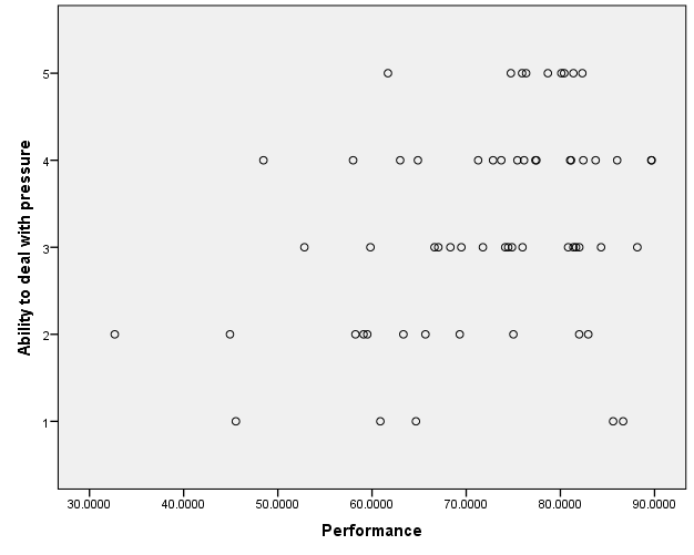
The chart above is a scatter plot illustrating the correlation between athletes’ performances and their ability to deal with pressure. There seems to be some form of relationship between the two variables. It can be seen that the higher an athlete’s performance, the better the athlete’s ability to deal with pressure. However, it is easy to observe that some of the points in the scatter plot do not follow this pattern. This is an indication that even though performance is related with an athlete’s ability to deal with pressure, the relationship may not be significant (Leedy, Ormond, & Silverman, 2012).
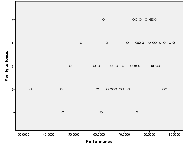
The scatter plot above is an illustration of the correlation between athlete’s performance and the ability to focus. There is obviously a relationship between the two variables. It may be observed that the higher an athlete’s performance, the better the athlete’s ability to focus. Even though there are some points that do not follow the trend, these points are less than the outlying points observed in Figure 1. This is an indication that the relationship between athletes’ performance and their ability to focus is significant. Therefore, athletes will perform better if they develop their ability to focus.
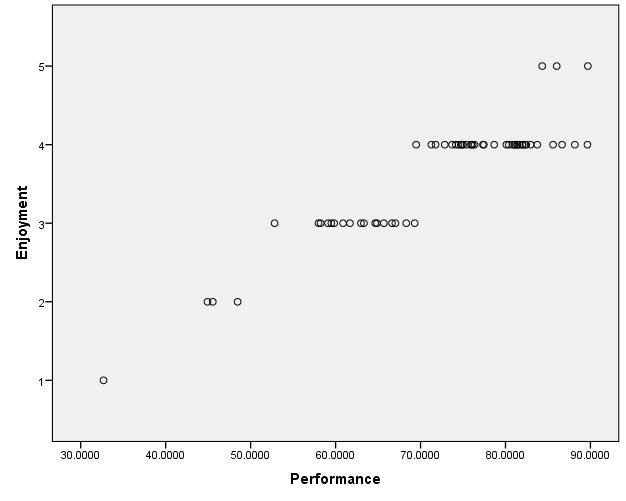
The scatter plot above is an illustration of the correlation between athletes’ performances and the way they enjoy the game. The scatter plot presents a clear indication of the relationship between athletes’ performances and the way they enjoy the sports. The trend is very clear and shows that the performance of an athlete is proportional to the way the athlete enjoys the game. It is very clear that the higher an athlete’s performance, the better more the athlete enjoys the game. All the points in the scatter plot follow a specific trend and the illustration shows a linear correction between the athletes’ performances and enjoyment. It can be concluded that there is a significant positive relationship between athletes’ performances and the way they enjoy a sport. Therefore, athletes will perform better if they enjoy the sports.
Chi-Square Test
A Chi Square test will be used to investigate the influence of an athlete’s level on the athlete’s ability to manage pressure, focus, and overall enjoyment of the sport (Thomas, Nelson & Silverman, 2011). The Chi Square can be used to test this relationship because the variables are categorical and consist of more than one independent group (pro, college and high school) (Jaynes, 2007). The current variables fulfill these two assumptions and this makes the Chi Square test applicable. The following tables are the results of the Chi-Square test.
Group * Ability to deal with pressure.
The table above shows that pros have the highest ability to deal with pressure, followed by college athletes, and finally high school athletes.
The X2 = 25.531 and P = 0.001. This indicates that there is a statistically significant relationship between group and ability to deal with pressure (Kline, 2004).
Group * Ability to focus.
The results are similar to the previous crosstabs table.
There is a statistically significant association between the variables.
Group * Enjoyment.
The results are similar to the previous crosstabs results.
There is a statistically significant relationship between the variables.
Conclusion
The main finding of the research is that an athlete’s level affects the athletes’ performance. Not all the three statistical tests performed were required to draw this conclusion. The Chi Square test and the correlation/regression tests would have provided sufficient evidence regarding the influence of athletes’ levels on their performance.
References
Bluman, A. G. (2012), Elementary statistics: A step by step approach. New York, NY: McGraw-Hill.
Jaynes, E.T. (2007). Probability theory: the logic of science. Cambridge: Cambridge Univeristy Press
Kline, R. (2004). Beyond significance testing: Reforming data analysis methods in behavioral research. Washington, DC: American Psychological Association
Lane, D. M. (2005). HyperStat online statistics textbook. Web.
Leedy, P., Ormond, J. E., & Silverman, S. J. (2012). Practical research: Planning and design. Columbus, OH: Merrill-Prentice Hall.
Thomas, J. R., Nelson, J. K., & Silverman, S. (2011). Research methods in physical activity. Champaign, IL: Human Kinetics.