Long-Term Trends of Commodity Prices From 1900 to 2011

Abstract

This dissertation aims to check the long-term movements of primary commodity price indexes. The data used in this project is the updated version of the index introduced by Grilli and Yang (1988). This new version covers the period from 1900 to 2011 including four kinds of price with two approaches of algorithm. The regression part applies to two time series model called ARMA and ARIMA models. To ensure the ARIMA models are correctly specified, we employed unit root tests to determine the order of integration of the data. The results suggest that the ARIMA models chosen provide adequate conditional characterisations of the various commodity price indexes. Commodity prices cannot be perfectly forecasted due to the impact of growth and technology.

Introduction

This dissertation aims to analyse the commodity price indexes for the different periods in the history of worldwide commerce and trade between developed and developing countries. The various periods represent years where those basic commodities were traded and bought for personal and public consumption. The study of commodity price trends demonstrates the flow of supply and demand during those periods which, as this law suggests, affects prices. While the law of supply and demand does not change and remains all throughout the different historical periods, it is also dependent on the way commerce and trade is practiced in those times.

The main focus is on prices of primary commodities from developing countries and manufactured products of developed countries. Quite a number of theories have been studied and related to the PS hypothesis and its effects on economic policies. Some economists provided evidence but these were argued upon by others who noted the gaps in the indexes.

The results of the indexes do not positively show that supply and demand affect the commodity prices; therefore, it is necessary that we examine the indexes that provide evidence for the hypothesis that there is a downward trend in the NBTT despite the fact that the flow and supply of prime commodities is continuous. The downward trend affects economies and economic policies for both developed and developing countries. The factors in the NBTT decline are clearly discussed in the literature.

Evidence from the literature suggests that the distribution of gains from production affected the long-run trends in the NBTT of trading countries, from developing to developed countries, which influenced the distribution of increases from trade between commodity producers in developing countries and consumers in developed countries.

In the data analyses, we explored the price indexes of various economic researchers and international agencies and the declining trend of prices of primary commodities from 1900 to 2011. We paid particular interest to the Grilli and Yang’s (1988) index, which was used in the allocation of growth between producers (the developing countries) and consumers (the industrial countries), although their indexes focused on the period 1900 to 1986. The indexes used had gaps, which point to the two world wars, but were filled up by Grilli and Yang by way of interpolation.

The renewed interest in the Prebisch-Singer hypothesis is primarily due to two factors. First, Grilli and Yang (1988) introduced new computed commodity price indexes which start from 1900 to 1986. The second factor is that there has been a reassessment of the evidence due to the introduction of new methods in analysing time-series data.

The starting point for Grilli and Yang’s work is their conviction that having high quality price indexes is essential when testing the PS hypothesis. Using their new commodity index, Grilli and Yang re-estimated the time trend model and found a statistically significant long-term decline in the NBTT that supports the Prebisch-Singer hypothesis. According to this hypothesis which came out of independent studies of Rual Prebisch (1950) and Hans Singer (1950), the prices of primary commodities and manufactures have a downward trend over a certain period.

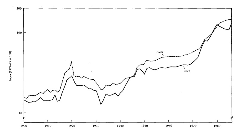
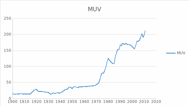
The PS hypothesis, which predicted the declining trend of commodity terms of trade, is near or almost similar to the actual terms of trade, as shown in figure 1. Grilli and Yang’s (1988) new computation of commodity price indexes triggered the reassessment of the hypothesis evidence.

Over the years, empirical analyses of commodity price trends have proliferated. Few hypotheses in development economics have not attracted as much attention as the PS hypothesis. Spraos (1980) was among those to rekindle academic interest in the empirical validity of the PS hypothesis in the late 1970s.

In an extension of Spraos’ work, Sapsford (1985) found evidence of discontinuous changes in the commodity price data used by Spraos. But Sapsford (1985) found ‘structural instability’ in Spraos’s work, and argued that the latter’s findings were misleading.

New empirical studies on the PS hypothesis have emerged and so economists continue to debate about it. Cuddington and Urzúa (1999) noted that all these studies appeared to have overlooked the importance of the serial correlation reflected in the price series. The Structural Time Series approach has been proposed by Harvey and others in a number of papers (Harvey and Todd 1983; Franzini and Havey, 1983; Harvey, 1985; Harvey and Durbin, 1986). This approach requires no preliminary assumptions about the properties of the series. Cuddington and Urzúa (1999) re-evaluated the Grilli-Yang index, and focused on the requirement that the error processes in the estimated time trend models be stationary.

Perron (1990) has also examined the (MUV-deflated) Grilli-Yang commodity price index (GYCMPI) for 1900-1983 for the presence of a unit root. Von Hagen (1989) took a different approach from Cuddington and Urzúa (1999). At the same time, the role of commodity prices as foundations of inflation has been referred to significantly and widely in the literature, with many different outcomes.

This dissertation has four parts. The first part explored the literature focusing on the background, concepts and meanings of commodity price indexes in the different periods. The second part lists some information about the data used in this project. The models ARMA and ARIMA comprised the methodology part along with the root tests. The last part is the result of stationarity of each index, fitting model for each index and some forecasts.

The ARMA and ARIMA models appeared in the regression part. An important step was to check the stationarity of the data by applying unit root test. In selecting the appropriate time series model, it is important to correctly capture the time series behaviour of the data. We employed the Akaike and Schwarz information criteria to assist in determining the correct AR and MA lag lengths in our time series models.

The stochastic behaviour of commodity price plays an important role in evaluating commodity-related projects. There are many aspects of commodity price indexes which were analysed, for instance, the variance and skewness, the volatility, the relationship between these indexes with other important economical indexes, and the trend of these indexes during the time periods of commerce and trade. The commodity price index tells us the price elasticity of the various commodities in the different periods, ranging from food to basic needs to raw materials for product manufacturing, etc.

Knowledge of commodity prices and analysing indexes help policy makers institute policies to pre-empt crises and deal with economic crises. Ordinary citizens should also learn to understand commodity price indexes as these are connected with daily life.

Literature review

Rual Prebisch (1950) and Hans Singer (1950) have independently claimed that several factors would combine to construct a worldly decline in the relevant primary commodity prices in terms of manufactured goods. This has been popularly known as the PS hypothesis, the subject of several empirical researches, and has influenced economic policies of developed and developing countries. The policies aimed to differentiate their productive constructions and export bases away from primary commodities towards manufactured goods, thereby evading the terms of trade deterioration Prebisch and Singer (1950) warned about. The factors in the commodities price decline are discussed in the data and methodology sections.

Over the years, researchers have provided empirical analyses of commodity price trend based on the PS hypothesis, but many hypotheses in expansion economics have not drawn as much attention as the PS hypothesis. Most of the empirical arguments about the PS hypothesis have concentrated on the non-stationarity of real commodity prices, which take the form of a non-random trend, a stochastic trend, or with the structural jumps in the trend. The original empirical surveys of Prebisch and the United Nations (1949) reinforced the theory. The evidence collected during the 1950s, 1960s, and 1970s, which has indicated continual upgrading in the quality of available commodity and manufacturing price indexes and more complex econometric techniques have been mingled. John Spraos (1980), Grilli and Yang (1988), Cuddington and Urzúa (1999), and D. Sapsford (1995) have investigated, made their own analyses of the deteriorating trend from the indexes of international agencies, and provided conclusions, albeit, mostly depended on the PS hypothesis.

Spraos (1980) critique of the P-S hypothesis

At the start of his analysis, Spraos (1980) made an intriguing contention about the Prebisch-Singer hypothesis: that economist Prebisch (1950) lacked statistics (or there were gaps in the index) that forced him to depend on index of a particular country, Britain. The prices of traded commodities did not distinguish where the products originated. This is his first contention, only to retract later and then support the theory that there is really such a trend but with exaggerated statistics from Prebisch.

Spraos (1980) argues that Prebisch (1950 as cited in Spraos) only depended on the statistical data of the United Kingdom, and from this he cut two overlapping indexes to cover the periods 1876 to 1880 and 1946 to 1947, showing data improvement for Britain. The Spraos (1980) evidence states that since Britain, a major product manufacturer at that time, was showing “secular improvement” the trend reflected a world-wide NBTT decline. The hypothesis has been greatly criticised because of the gaps in the series. Prebisch argued that his data came from the UN (1949), which proved that his data was not original (Spraos 1980).

Spraos (1980) enumerates four major arguments against Prebisch’s (1950) hypothesis:

1. The NBTT data for the United Kingdom could not be translated as those from the industrialised world; thus, the opposite could not be considered representative of the terms of trade of primary commodities (Spraos 1980);
2. Developed countries also produced and exported primary products for industrialised countries, not only those coming from developing countries (Meier & Baldwin 1957; Meier 1958; Van Meerhaeghe 1969; Frank 1976 cited in Spraos, 1980).
3. The rise in the United Kingdom’s NBTT could be attributed to reduction in transport expenses and not to the decline in the prices by primary producers since exports were valued or priced based on prices quoted for delivery in London, Liverpool (Viner 1953; Baldwin 1955; Ellsworth 1956; Meier & Baldwin 1957; Meier 1958, 1963 as cited in Spraos, 1980).
4. New manufactured products were exported while the existing ones were upgraded, but these were not clearly stated in the price index of manufactures, which provided an upward bias that vaguely created the impression that NBTT of primary products was declining (Viner 1953; Baldwin 1955, 1966; Ellsworth 1956; Meier & Baldwin 1957 as cited in Spraos, 1980).

Relying on these data, Spraos (1980) argues that while the deteriorating trend can be seen, it is not as large as suggested by the Prebisch’s (1950) series. He further contends that the evidence contrary to the PS hypothesis can be seen on the 1870 to 1938 data, but the declining trend is more doubtful when the period is extended forward. Moreover, index numbers formulated many years back have “conceptual problem errors of measurement” (Spraos 1980, p. 109). The question is whether the available series can plausibly represent for the questionable NBTT or can clarify the plausible conclusions derived from those representations.

Spraos (1980) then provides regressions aimed at testing whether such a trend is reflected in the data and thus support the assumptions acquired by visual analysis of the time series. The analysis is not to provide explanation over the long-term movement of the terms of trade (given that it could produce high R²s), not even to acquire ‘efficient predictors’, nor ‘to seek the best fit on time’ (Spraos 1980, p. 109). He then makes a semi-loglinear regression to show a measure of trend, given that the coefficient of t provides the ‘average rate of change of the regression per unit time given implicitly in the data and the symbol of coefficient clearly tests the hypothesis of deterioration’ (Spraos 1980, p. 109).

Spraos (1980) then investigates Britain’s representative NBTT for industrialised countries. Some reliable author-economists, like Martin and Thackery (1948 as cited in Spraos) and Kindleberger (1956 as cited in Spraos), also investigated the combined NBTT of industrialised countries and reported that there was no significant trend in their NBTT up to World War II. During the same period, there was no significant trend reported for the US NBTT and for industrial Europe with respect to imported primary products and exported manufactures.

Spraos (1980) produces a table, representing the League of Nations series, which has a compilation of world trade data. The purpose of this table and analysis is to examine whether Prebisch (1950 as cited in Spraos, 1980) gravely misled himself and the economic world by not using an accurate evidence for his hypothesis. By using log regressions of the series on t, the Prebisch series provides ‘an annual rate of change of the relative price of primary products’ which is –0^.9 percent, and the League series is –0^.6 percent. The analysis presents evidence that there is an exaggeration in Prebisch’s data but this is also present in the League’s series.

According to Spraos (1980, p. 253), Lewis (1952) improved the League’s data by adding ‘the prices of imports and exports of manufactures of the United States and in other ways’. The League’s series shows robustness, and the UN Secretariat added conceptual homogeneity. Based on the data collected by Spraos (1980), Britain’s NBTT as basis for relative price of primary products with respect to manufactures in world-wide trade ‘was not misleading as to direction though it gave an exaggerated impression of the magnitude of deterioration’ (Spraos 1980, p. 113). Britain, which was the leading world trade country at that time, had a large and improved NBTT (Spraos 1980).

Spraos (1980) has made thorough analyses of the deteriorating trend for the 70 years up to World War II and provided a conclusion that indeed there was evidence of the trend in the relative price of primary products. However, there are reservations pointing to the quality of the evidence, although the finality of the conclusion is reached when he examined one by one the main points taken in questioning the inference of the deteriorating trend. He, however, discovered that Prebisch (1950) exaggerated the rate of deterioration – ‘at worse by a factor of more than three’ (Spraos 1980, p.126).

The Grilli and Yang (1988) index

Grilli and Yang (1988) focus on long-term run of prices of primary commodities, and their index has become one of the most sought-after sources on the subject. Their main concern is to analyse the price movements but not to provide economic explanations over this phenomenon. They start with their initial finding that having high quality price indexes is necessary when testing the PS hypothesis. The authors provide data on the prices of nonfuel commodities. They compare the statistical properties between the movements in those commodities and the manufactured products. After this examination, the author-economists further investigate the potential consequence of development on the commodity prices.

Grilli and Yang (1988) modified the United Nations Index in what became known as MUVUN (Manufactured Unit Values, United Nations) based on the Economist Index (EI) and the Lewis Index (WALIl), then used this to analyse 24 nonfuel product prices. They used the 1977-1979 data as weights. The new index – the GYCPI – tells of the movements in different periods of primary commodities. The index filled the two gaps (1914 to 1920 and 1939 to 1947) in the price index by way of their adopted strategy of ‘interpolation,’ utilising product values of the United States and the United Kingdom during the period, as indicators.

Grilli and Yang further re-estimated the time trend model using their new commodity index and found a statistically significant long-term deterioration in the NBTT. Their econometric analysis focused on the likelihood of first-order serial correlation and structural breaks, noting that ‘examination of the residuals of the semi-log time regressions, as well as a priori knowledge of the exogenous factors that may have caused a structural break in the price series, indicated the possibility of breaks at three points in time: 1921, 1932 and 1945’ (Grilli & Yang 1988, p. 10). At this time, we can conclude that the modified index (MUV) is more reliable as Grilli and Yang filled the gaps to provide a complete data for the 1900-1986 deteriorating trend of the NBTT of primary commodities and manufactures between developing and developed countries.

The researchers also developed another index of domestic prices of products made in the United States (example: energy, timber, and metal), as they wanted to avoid the overlapping of goods in the indexes. The index is used to provide a concept of the connection between ‘prices and unit values of exports’ of the different periods and of the logic of the results taken from the interpolation they have created to fill the gaps (Grilli & Yang 1988, p. 5). The two indexes now provide a relative trend growth for the period (1900 to 1986), equivalent to 2.49 percent annually for the MUV (this is shown in figure 1). The USMPI has exhibited 2.48 percent a year. However, the authors argue that the MUV is a bit erratic compared to the USMPI. The MUV has a ‘percentage deviation from trend’ of 6.2 percent for the 1900 to 1986 period, while the USMPI only got 5.1 percent. (Grilli & Yang 1988, p. 5)

The two indexes were taken to calculate two collections of relative prices of primary commodities (nonfuel). The first set of commodity prices calculates the beginnings of the purchasing power of those primary commodities which were traded domestically; thus, their prices were also domestic.

Cuddington and Urzúa’s (1999) critique

Cuddington and Urzúa (1999) examined the NBTT downward trend and the Grilli and Yang (1988) index. The authors applied the “time series methods” and discussed the cyclical characteristics of commodity prices using the Beveridge and Nelson (1981) technique. The interest in the cyclical movements in commodity prices is founded on the principle that in policy making the scope, length, and form of the cycles are as important as the current long-term trend.

In examining the NBTT downward trend, Cuddington and Urzua (1999) used the Grilli-Yang commodity price index (GYCPI) which, as mentioned earlier, explored 24 non-fuel commodities as weights and built a new index due to the gaps in the series, as discussed earlier. The GYCPI provided a picture of the significant drop in the NBTT and the other commodity prices examined by their index. Thirlwall and Bergevin (1985) also noticed the drop when they used the United Nations data from 1954 to 1982. Cuddington and Urzúa (199) found the advantage and relevance of Grilli and Yang’s (1988) index as all the other studies ignored the relevance of the serial correlation shown in the price movements.

Moreover, Cuddington and Urzúa (1999) found that the GYCPI was the most logical to use because the other used indexes – the World Bank, UNCTAD and IMF – lacked data as they applied only the periods after the war. On the other hand, the Economist Index (EI) had also been applied with several revisions and its weights are founded on the relevant trade of industrial countries instead of the worldwide import weights. The GYCPI used an annual index of manufactured goods unit values, also called MUV-GY. This series matches with the index of unit values computed by the equivalent United Nations manufactured goods unit values, or MUV-UN, which had gaps. Grilli and Yang filled the gaps through interpolation.

The NBTT sequence taken through deflation of GYCPI by MUV-GY produces the index of real commodity prices used by Cuddington and Urzúa (1999). The series is denoted y(t) in Cuddington and Urzúa’s analysis and considered as good as the others, but they noted that the MUV-GY does not have power on possible changes in the quality of either manufactured goods or primary commodities. This is one of the problems noted in the literature, where quality changes cannot be taken into account in the measures of real commodity prices. Cuddington and Urzúa (1999) have cited Grilli and Yang’s (1988) remarks on the possibility of an “upward bias” borne by manufactured goods prices as they integrate the advantages of technological development that might have improved the goods’ quality (Cuddington & Urzúa, 1999).

All the other studies, excluding Grilli and Yang’s (1988), failed to provide statistical details of the univariate illustrations of the price movements that represented the different years. In other words, all those suppositions had regression difficulties.

Cuddington and Urzúa (1989) considered the price movements as nonstationary. In their analysis of GYCPI, they rebuffed the doctrine of determinism and supported the stochastic trend model using the test methods of Dickey and Fuller (1979), along with the method of Perron (1988). Here, Cuddington and Urzúa (1999) concluded that there was no deterioration in the NBTT for the period from 1900 to 1983. When they focused on the statistical problems caused by non-stationary, they reached a conclusion that there was no significant secular deterioration in the relevant commodity prices. They supported the Grilli and Yang finding that the significant deterioration in commodity prices vanished when the latter considered the TS specification and the large break in the data after 1920 (Cuddington & Urzúa 1989, p. 441). In their examination of the residuals from simple TS and DS models, they concluded that there was a gap in the Grilli-Yang index after 1920, in which Grilli and Yang explained that the data breaks referred to ‘exogenous’ events. The sharp drop in prices after World War II explains the adjustment in commodity supplies and demands following the war. They also quoted Friedman and Schwartz’s theory in the belt-tightening policies of the Federal Reserve in 1920. The literature provides statements that in real terms, commodity prices exhibit invisible or definitely dropping movements, but there are indications of long term drops. Deaton (1999) argues that although the trend is erratic, we also see variance.

Cuddington and Urzúa (1999) concluded that the Prebisch-Singer hypothesis should be applied with changes: that primary commodity prices relative to manufactures had a sharp drop after 1920. It is a one-time drop and there is no continuing downward trend in the prices of primary goods. According to Cuddington & Urzúa (1999, p. 441), it is inappropriate to describe the movement of real primary commodity prices since the turn of the century as one of ‘secular deterioration’. But, indeed, Cuddington and Urzúa recognized that there is a downward trend which supports the other studies, although the disagreement is on the period the trend stopped.

One worrying feature of the Cuddington-Urzúa (1999) paper is their ad hoc methodology for separating structural breaks. It was Cuddington and Urzúa’s examination of the residuals from simple TS and DS specifications that led them to the result that there was a gap in the Grilli-Yang index after 1920. This “data snooping” might not be good because it leads us to choose a point with a high Chow-test value. To be strict, Perron’s statistical test for unit roots in the presence of a shift in the mean needs that the event be exogenous which ensures it is no problem to take it out of the stochastic process when generating the data.

Cuddington and Urzúa (1989, p. 429-430) admitted that ‘in light of its critical importance in our findings below, this sharp drop in prices cries out for some explanation… Presumably, it reflects the adjustment in commodity supplies and demands following the end of the First World War.’ They went on to paraphrase Friedman and Schwartz’s discussion of the belated tightening in Federal Reserve policy in 1920. Unfortunately, the conclusion regarding the trend in commodity prices seems to hinge critically on whatever the break is taken into consideration in the time series analysis.

The DS and TS models

The TS model suggests that ‘all price fluctuations around the deterministic trend line (which has a zero slope here) should be viewed as cyclical; the deterministic trend reflects changes in the permanent component of prices’ (Cuddington & Urzúa 1999, p. 438). The DS model provides a ‘decomposition of price innovations into permanent and cyclical components, with the former being stochastic rather than deterministic’.

Sapsford (1985) evidence

Sapsford (1985) criticised Spraos’s (1980) analysis and conclusion of the PS hypothesis regarding NBTT declining trend. Sapsford’s analysis also supports the PS hypothesis, but at the same time, he criticises Sprao’s methodology as having statistical problem. Sapsford’s (1995) methodology drew a simple trend model from the methodology used by Spraos:

NBTT_t = a + rt + u_t (t = I, …, n)

By using regression methods, Sapsford (1985, p. 782) provides the ‘long-run trend of growth in the NBTT’. He is critical of Spraos’s support of the PS thesis for the pre-World War II period which was acquired by using fitting model (I) by means of the ordinary least-squares (OLS) to two of the series, the United Nations series, which included the 1950 to 1970 period, and the World Bank index (post 1950 period). Sapsford criticised Spraos’s method of trend analysis and estimation, saying that it is only applicable on the premise that the primary constraints of the NBTT’s growth direction remain unchanged during the analysis of the index (Sapsford 1985, p. 782).

Sapsford (1985) found evidence of discontinuous changes in the Spraos’s commodity price data. He observed the structural instability and allowed ‘intercept and slop dummies in 1950,’ allowing him to conclude that there was evidence supporting the PS hypothesis for the pre- and post-World War II periods.

In his study of Spraos’s (1980) analysis, Sapsford took note of the equations provided in a table stating the Cochrane-Orcutt (C-O) counterparts and Spraos’s regressions. The OLS or the C-O equations, made to provide the structural instability in the growth during the pre and postwar periods, results from the data provided by Spraos which created the 1900 to 1970 negative and significant growth rate which supports the PS hypothesis. (Sapsford 1985, p. 783)

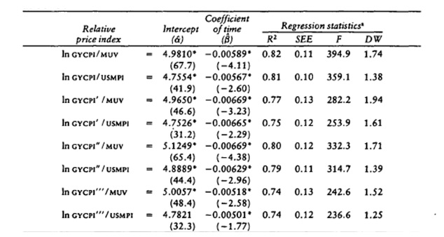
Table 1 shows Spraos’s regression analysis. Absolute t values are presented in the figures in parentheses; the single asterisk represents the ‘coefficient which is significantly different from zero at the 5 percent level’. NBTT₁ represents the UN series, which is updated to 1980 with data taken from the United Nations Statistical Yearbook (1981 as cited in Sapsford, 1985). The results of the Spraos series support the P-S hypothesis: there is an upward trend before the war and a downward trend after the war, which shows a similar trend during the 1900 period up to the outbreak of the Second World War. However, Sapsford (1985) notices that the UN results provide a different trend. The equation does not show significant alteration in the intercept term but an upward trend after the war. The upward movement also shows that it cannot change the negative trend. The equation further shows that ‘the restriction that the trend growth rate in the UN series and the coefficient of D₈ sum to zero in (I.12) is rejected at the 1% level on the usual t test’ (Sapsford 1985, p. 786), which creates evidence to support the PS hypothesis. This further provides a negative trend for both the pre- and post-war periods.

In the final analysis on Spraos’s series, Sapsford (1985) concludes that there is ‘structural instability problems’ in Spraos’s analysis when he provided a re-estimation of Spraos’s own equations from the data provided which showed that there was ‘trendlessness for the period 1900-70’ (Sapsford 1985, p. 787). Although Sapsford recognises his limitations with respect to his analysis and that of Spraos, he continues to conclude that ‘Spraos’s earlier findings were misleading’ (Sapsford 1985, p. 787).

Data

Grilli and Yang (1988) explored the 24 non-fuel price indexes and the modified index, because they wanted to provide a complete index that would not only examine the post-World War II period but also the periods before the war. The World Bank index started with the 1948 period and beyond while the United Nations index had gaps.

Since it is unfeasible to create a new price index of manufactures that date back from 1900, they used a modified form of the MUVUN (Manufactured Unit Values, United Nations), which they constructed by interpolation to satisfy the continuity, taking both import and export unit value of manufactured goods of the United States and the United Kingdom as indicators. The authors achieved the interpolation by taking average values of the sub-indexes and by using the estimated equation to generalise the values of the MUV index. For the period from 1915 to 1920, the researchers succeeded in conducting interpolation by first order regression of the MUV index with the import and export unit values of manufactures indexes of the United States and the United Kingdom.

Some variable weights reflected the relative significance of the various types of manufactures in international trade. The GYCPI is often referred to and discussed by economic researchers. Additionally, Grilli and Yang (1988) built sub-indexes for agricultural food commodities (GYCPIF), non-food agricultural commodities (GYCPINF), and metals (GYCPIM). The value of the weights relies on each product’s standard price for the period. These data have been used in many different situations in later researches (Bleaney & Greenaway 2001; Kimet et al. 2003).

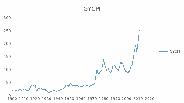
Important sources used by Pfanffenzeller, Newbold and Rayner (2007) provide more information on the commodity price data, such as the World Bank Development Prospects Group’s CPI, the IMF price tables, and the OECD database. Most of these data can be retrieved through the respective organisations’ websites. Grilli and Yang (1988) have to combine one or two indexes because of the incompleteness of the data. This creates some problems, and a challenge to the researchers, because finding a perfect match in the data is really difficult to do. The GYCPI is displayed in Figure 2.

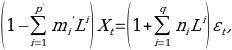
Stephan Pfaffenzeller, Paul Newbold, and Anthony Rayner (2007) maintain that the composite index defined by Grilli and Yang (1988) is computed as a weighted average of the commodity prices, which is:

where n=24, a_i is ‘the appropriate commodity weight,’ and P_i,t is the price of commodity i in period t, catalogued to 1977-1979 mean. Cuddington and Wei (1992) suggested that it may be better to use a geometric aggregation to define the index which is expressed as:

Cuddington and Wei (1992) discussed the specific features of this alternative index in details. ‘Manufacturing unit value index’, referred to in Cuddington and Wei (1992), is taken to reinforce the GYCPI, now termed MUV-G5 index. It is an index for the G5 countries that it is also used by the World Bank, but regarded as unsuitable measure for imports of developing countries, although it is assumed that it can be used as index for imports of developing countries. The MUV is used to measure manufactured products. This is referred to in the MUV 15 index, or the 15 countries.

The indexes are the equivalent to the total of each country’s exports, and the parts are calculated using the SITC tool for exports. In the manufacturing sector, Grilli and Yang (1988) used the OECD Producer Price Index (PPI). The respective countries’ relative weights have different percentages, as shown in table 1.

The MUV5, representing France, Germany, Japan, the United States and the United Kingdom, has another set of data. The World Bank maintains that the time horizon and frequency used in predicting the MUV (15) are the same with the data used in the commodity price prediction.

The MUV receives regular updates so that the data coincide with the Global Economic Prospects and other predictions. The World Bank, through its agency the Development Prospects Group, also provides updates. Grilli and Yang (1988) regularly use the 1977-1979 averaging value with 1990 as base year.

Nonfuel commodity prices have lagged behind even during the early 1900s compared to those of manufactures in the United States and the rest of manufactured products coming from industrial countries. These are considered, or noted, in the BYCPI and USMPI series as these showed a negative exponential trend of 0.57 percent a year over the 1900 to 1986 period. On the other hand, the GYCPI and MUV series exhibits a trend decline of 0.59 percent a year over the same period. This is shown in the figure below.

The GYCPI shows that the purchasing power of nonfuel primary commodities in terms of manufactures dropped since 1900 at an annual rate of 0.63 percent to 0.67 percent when the situation arises that the USMPI or MUV is made to gauge the manufactured goods prices. In including the fuel prices in the index with the use of the GYCPI, the decline fell to 0.52 percent annually. The prices of primary commodities and nonfuel commodities dropped on trend since the period 1900 to 1986.

In checking for the stability of the estimated time coefficients of Grilli and Yang’s (1988) indexes (GYCPI/MUV and GYCPI’’’/MUV regressions), they tested for ‘the possibility of a change in slope’ through regression used by Suits, Mason and Chan (1978 as cited in Grilli and Yang, 1988, p. 10), in order to approximate the time trend of the indexes. Grilli and Yang found ‘no clear break’ that occurred since the 1900 period. World War I made a mark on the cyclical instability in commodity prices which showed in the first forty years covered by the Grilli and Yang series.

Grilli and Yang (1988) also computed the trends in the prices of the three categories of primary commodities relative to those of manufactures, such as for food (GYCPIF), non-food agricultural raw material prices (GYCPINF), and metal (GYCIPIM). They found that the decline in the relative prices was not uniform. The long-term decline showed in the metal and non-food agricultural product prices. In other words, not all producers of nonfuel primary commodities did feel the relative prices fall ‘in the purchasing power of a given volume of their products over the past eighty-six years’ (Grilli & Yang 1988, p. 11).

The commodity price indexes that include the Grilli and Yang (1988), the MUV, GYCPIM are incorporated in a long table shown in Appendix 1.

Methodology

The aim of the research is to investigate the long-term behavior of commodity prices. In order to achieve this aim, several time series analysis models were used.

Unit Root Test

Two characteristics of ‘economic time series’ are known as ‘trending behavior and non-stationarity’ (Grilli & Yang 1988). These two also influence financial time series.

Any inference based on a misspecified model may be misleading unless the model is correctly specified. A necessary first is to determine the order of integration of the data, which may be achieved using a unit root test. Moreover, it will also assure appropriateness of model chosen to make more accurate predictions. Among numerous methods to test unit root, there is a well-known one which is called augmented Dickey-Fuller (ADF) test, popular to be used in more complicated models for time series. The procedures are introduced in the following part. Assume autoregressive model about time series y_t as below:

(XX)

where α is the drift, β is the coefficient associated with the linear deterministic trend and k is the lag order.

The augmented Dickey–Fuller test is on the basis of statistic related with the significance of negative coefficient γ. The null hypothesis is that the data in question has a unit root. This may be expressed as:

H0: gamma = 0 in equation no. (XX)

The alternative hypothesis is expressed as:

H1: gamma < 1 in equation no. (XX).

The ADF test is calculated using:

(XX1)

In (XX1) gamma hat and SE (gamma hat are obtained from OLS estimation of equation (XX).

DF_τ is smaller than the critical value related at a given confidence level, null hypothesis gamma = 0 will be rejected, implying that there is no evidence of a unit root in the data of interest. In addition, before calculating DF statistics, lag order k should also be determined. If the lag order k is incorrectly specified for equation (XX) then inference about the presence of a unit root based on tests constructed as (XX1) may be invalid.

The delta coefficients in (XX) have to be correctly determined. One approach is to begin with a high order for k and to test down until the kth lag coefficient is significant. However, most serious disadvantage is that higher lag order seems to be preferable by this method without considering appropriateness and complexity of the model.

Therefore, there is also another feasible approach to measure relative quality of model with certain lag order by trading off complexity and goodness of the model, such as Akaike information criterion (AIC) or Bayesian information criterion (BIC). In this project, Akaike information criterion (AIC) will be applied to estimate lag order k, which can be represented by the following equation:

(XX2)

where k is lag order and L is maximized likelihood of statistical model. It can be seen that AIC offers a relative estimate of complexity increase by lag order k and information lost by likelihood L, which provides the assumption that AIC is more appropriate.

In addition, EViews has been chosen as the statistic software for this project. EViews can easily give the result whether the data has unit root. If the data rejects the null hypothesis, it means the data does not have a unit root. If EViews accepts the null hypothesis, it indicates that the data itself is nonstationary. When the data does not have this property, we can also test if its first order difference has stationarity. Once we have the result about the stationarity of the data, we can do the regression model. For the stationary data we will apply ARMA model, and ARIMA model will be used for the nonstationary data.

ARMA model

ARMA is acronym for autoregressive moving average model, which was first defined by Peter (1952) to aid in mathematical analysis, particularly econometrics. Hannan and Deistler (1988) also gave their expertise, using the Box-Jenkins method. ARMA can be used to describe a stationary time series, and to predict future values, using a time series of two parts, ‘the autoregressive and the moving average’ (Grilli & Yang 1988). This is represented in the symbol AR(p) , and calculated using the formula:

The formula has the following representations:

as coefficients, c can be considered constant, while ε_t represents the random variable. Considering moving-average model, the one with order q, noted by MA(q), can be written as:

where

are white noise error terms,

are the corresponding coefficients of error terms and μ is drift part.

RMA(p, q), has the following equation.

Equivalently, ARMA model can also be specified by lag operator L. By these simplifying notations, the alternative AR(p) model is given by

and the alternative MA(q) model is given by

Thus, Box and Reinsel (1994) used a different method to estimate ARMA coefficients that allows ARMA to be similar expression as polynomial. Thus the ARMA(p,q) model could be expressed in

When suitable values of p and q are estimated, generally, ARMA models can be fitted by least squares regression to estimated coefficients in ARMA. ARMA p and q must have an appropriate data which can be taken from autocorrelation functions. AIC can be used to finding p and q as recommended by Brockwell & Davis (2009).

ARIMA

ARIMA is acronym for ‘autoregressive integrated moving average,’ considered an additional tool for ARMA. The difference between these two similar models is that ARIMA model is employed in some situations when data do not show stationary property, while an initial differencing method can be used to eliminate the nonstationarity. This is also referred to as ARIMA(p,d,q) model, wherein p represents the autoregressive order; d for the integrated order; and q for the ‘moving average order’ of ARIMA. ARIMA models come from the general ARMA model which is expressed in the following formula:

where L indicates the lag operator, the m_i are the autoregressive parameters of the model, the n_i are the parameters appearing in the moving average part and the ε_i  denote error terms. The term ε_t is considered a random and independent variable, taken from a ‘normal distribution’.

Assume now that the polynomial

 has a unitary root of multiplicity d which means that it can be rewritten as:

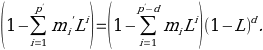
Doing the change of parameters with p = p’ – d will lead an ARIMA(p,d,q) model to such a formula:

Results

The stationarity of the data

The stationarity of GYCPI/MUV for the period 1900 – 1986

The result for examining the stationarity of GYCPI/MUV is illustrated in table 2. From this table, EViews gives the probability 0.1125 and t-statistic value for Augmented Dickey-Fuller test statistic with -3.095835 which is larger than 10% level. This indicates that there is no significance evidence against the null hypothesis of a unit root. This evidence suggests that there is a unit root in the level of GYCPI/MUV series.

Given the apparent unit root in the level of GYCPI/MUV, we will look at its first difference, denoted as D(GYCPI/MUV). Table 3 shows the result of checking stationarity of D(GYCPI/MUV). This evidence suggests that there is no unit root in the first difference of GYCPI/MUV series. This is consistent with the view that this series is I(1).

The stationarity of GYCPICW/MUV

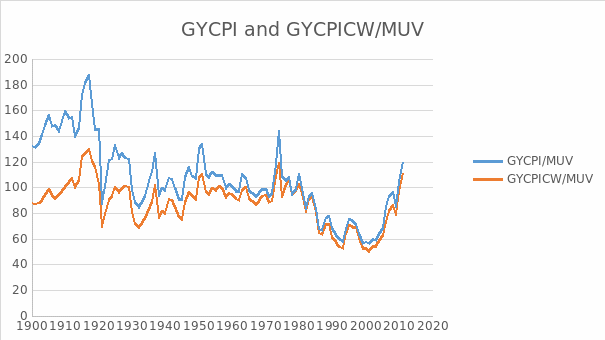
The result in examining the stationarity of GYCPICW/MUV is illustrated in table 6. From this table we can see EViews gives the probability 0.2128 and t-statistic value for Augmented Dickey-Fuller test statistic with -2.766571 which is larger than 10% level. There is no evidence against the null of a unit root in GYCPICW/MUV. The evidence is consistent with the view that the data are non-stationary.

Again, given the apparent unit root in the level of GYCPICW/MUV, we will look at its first difference, denoted as D(GYCPICW/MUV). Table 7 shows the result of checking stationarity of D(GYCPICW/MUV). The evidence suggests that there is no unit root in the first difference of GYCPICW/MUV. This is consistent with the view that this series is I(1).

The stationarity of GYCPIM/MUV

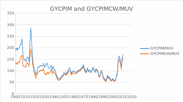
The result for examining the stationarity of GYCPIM/MUV is shown in the table 10. From this table we can see EViews gives the probability 0.4088 and t-statistic value for Augmented Dickey-Fuller test statistic with -2.339955 which is larger than 10% level. There is no evidence against the null of a unit root in GYCPIM/MUV. The evidence is consistent with the view that the data are non stationary.

Given the evidence of a unit root in the level of GYCPIM/MUV, we will look at its first difference, denoted as D(GYCPIM/MUV). Table 11 shows the result of checking stationarity of D(GYCPIM/MUV). The evidence suggests that there is no unit root in the first difference of GYCPIM/MUV. This is consistent with the view that this series is I(1).

The stationarity of GYCPIMCW/MUV

The result for examining the stationarity of GYCPIMCW/MUV is shown in table 14. EViews gives the probability 0.1549 and t-statistic value for Augmented Dickey-Fuller test statistic with – 2.937905 which is larger than 10% level. There is no evidence against the null of a unit root in GYCPIMCW/MUV. The evidence is consistent with the view that the data are non-stationary.

The evidence suggests that there is a unit root in the level of GYCPIMCW/MUV. If there is no evidence of a unit root in the first difference of the series this would be consistent with the view that this series is I(1). Table 15 shows the result of checking stationarity of D(GYCPIMCW/MUV). The evidence suggests that there is no unit root in the first difference of GYCPIMCW/MUV. This is consistent with the view that this series is I(1).

The stationarity of GYCPINF/MUV

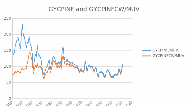
The result for examining the stationarity of GYCPINF/MUV is shown in the table 18. From this table, EViews gives the probability 0.0370 and t-statistic value for Augmented Dickey-Fuller test statistic with -3.571039 which is less than 5% level. There is no evidence of a unit root in the level of GYCPINF/MUV.

The stationarity of GYCPINFCW/MUV

The result for examining the stationarity of GYCPINFCW/MUV is shown in the table 21. From this table we can see EViews gives the probability 0.0214 and t-statistic value for Augmented Dickey-Fuller test statistic with -3.777520 which is less than 5% level. There is no evidence of a unit root in the level of GYCPINFCW/MUV.

The stationarity of GYCPIF/MUV

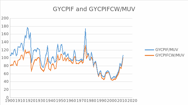
The result for examining the stationarity of GYCPIF/MUV is shown in the table 24. From this table we can see EViews gives the probability 0.0151 and t-statistic value for Augmented Dickey-Fuller test statistic with -3.901358 which is less than 5% level. There is no evidence of a unit root in the level of GYCPIF/MUV.

The stationarity of GYCPIFCW/MUV

The result for examining the stationarity of GYCPIFCW/MUV is shown in table 27. The result of 0.1211 can be taken from EViews and t-statistic value for Augmented Dickey-Fuller test statistic with -3.060341 which is a bit larger than 10% level. There is no evidence against the null of a unit root in GYCPIFCW/MUV. The evidence is consistent with the view that the data are non stationary.

Given the evidence of a unit root in the level of GYCPIFCW/MUV, we have to look at its first difference, denoted as D(GYCPIFCW/MUV). Table 28 shows the result of checking stationarity of D(GYCPIFCW/MUV). The evidence suggests that there is no unit root in the first difference of GYCPIFCW/MUV. This is consistent with the view that this series is I(1).

It is accepted among the storage model theorists that agricultural prices should be stationary. With an i.i.d. supply and a deterministic demand function, the storage model seeks to show how commodity storage induces price auto-correlation. Actually, under Prebish-Singer hypothesis, there exist some literatures having focused on stationarity of price. The primary reason why this phenomenon happened was the low income elasticity of commodity demand and the high prices caused by manufacturers’ market power. Policy also has effects on the price stationarity. It should be emphasized that there is obvious randomness regarding the existence of trends in agricultural commodities. Moreover, trends do not seem to sustain for very long time given the assumption of existence of trends. Since it is unknown that whether prices have trend, and whether price shocks are consistent, one reasonable solution at the level of producer and national may be extending commodity production, and this would probably diminish the risks connected with the existence of shocks and price volatility.

The regression

To get the regression model for each index, we should check the values of all the parameters first. For those indexes with stationary property, ARMA will be used for regression and for those indexes without stationary property, ARIMA will be implied. ARMA model needs two parameters p and q to be determined and ARIMA model needs three parameters p, d and q to be determined. There are some criteria which can be chosen to determine the parameter values. The Akaike information criterion (AIC) (Akaike, 1974) and Schwarz information criterion (SIC) (Schwarz, 1978) are two objective measurements to check the goodness of fitting for a model which takes those considerations into account. The order consistent of a criterionis described to be the criterion is minimized at the true order with a probability which approaches agreement as the sample size increases. The AIC procedure has however been criticized because of the inconsistence and tends over fitting models. Shibata (1976) demonstrated this for autoregressive models, Geweke and Meese (1981) for regression models, and Hannan (1982) for ARMA model.

The ARIMA model of GYCPI/MUV

The result of choosing parameters of ARIMA for GYCPI/MUV is shown in the table 4. The least AIC appears in ARIMA(1,1,1) with value 7.81. Table 5 gives the regression result for GYCPI/MUV. As we can see, the probabilities of C, AR(1) and MA(1) are all below 5%. This result means this ARIMA(1,1,1) fits GYCPI/MUV very well. Denotes GYCPI/MUV as ‘C’, then we have the following regression formula:

The ARIMA model of GYCPICW/MUV

The result of choosing parameters of ARIMA for GYCPICW/MUV is shown in the table 8. The least AIC appears in ARIMA(1,2,2) with value 7.09. Table 9 gives the regression result for GYCPICW/MUV. As we can see, the probabilities of AR(1) and MA(2) are both below 5%. This result indicates that this ARIMA(1,2,2)  model fitsGYCPICW/MUV well. Denotes GYCPICW/MUV as ‘CW’, then we have the following regression formula:

The ARIMA model of GYCPIM/MUV

The result of choosing parameters of ARIMA for GYCPIM/MUV is shown in table 12. The minimum AIC appears in ARIMA(0, 2, 3) with value 8.81. Table 13 gives the regression result for GYCPIM/MUV. As we can see, the probabilities of MA(1), MA(2) and MA(3) are all below 5% which means this ARIMA(0, 2, 3) fits GYCPIM/MUV very well. Denotes GYCPIM/MUV as ‘CM’, then we have the following regression formula:

The ARIMA model of GYCPIMCW/MUV

The result of choosing parameters of ARIMA for GYCPIMCW/MUV is shown in the table 16. The minimum AIC appears in ARIMA(1, 2, 2) with value 8.09. Table 17 gives the regression result for GYCPIMCW/MUV. As we can see, the probabilities of AR(1) and MA(2) are both above 5%. This result means the ARIMA(1, 2, 2) model does not fit GYCPIMCW/MUV very well. Denotes GYCPIMCW/MUV as ‘CMW’, then we have the following regression formula:

The ARMA model of GYCPINF/MUV

The result of choosing parameters of ARIMA for GYCPINF/MUV is shown in the table 19. The minimum AIC appears in ARMA (2, 2) with value 8.12. Table 20 gives the regression result for GYCPINF/MUV. As we can see, the probabilities of AR(1),AR(2), MA(1) and MA(2) are all below 5%. This result strongly means the ARMA (2, 2) modelfitsGYCPINF/MUV very well. This result means this ARMA (2, 2) fits GYCPINF/MUV very well. Denotes GYCPINF/MUV as ‘CN’, then we have the following regression formula:

The ARMA model of GYCPINFCW/MUV

The result of choosing parameters of ARIMA for GYCPINFCW/MUV is shown in the table 22. The minimum AIC appears in ARMA (1, 2) with value 7.43. Table 23 gives the regression result for GYCPINFCW/MUV. As we can see, the probabilities of AR(1), and MA(2) are all below 5%. This result tells us that the ARMA (1, 2) model fits GYCPINFCW/MUV very well. This result means this ARMA (1, 2) fits GYCPINFCW/MUV very well. Denotes GYCPINFCW/MUV as ‘CNW’, then we have the following regression formula:

The ARMA model of GYCPIF/MUV

The result of choosing parameters of ARIMA for GYCPIF/MUV is shown in the table 25. The minimum AIC appears in ARMA (1, 2) with value 8.24. Table 26 gives the regression result for GYCPIF/MUV. As we can see, the probabilities of AR(1) and MA(2) are all below 5%. This result indicates that this ARMA (1, 2) model fitsGYCPIF/MUV well. Denotes GYCPINF/MUV as ‘CF’, then we have the following regression formula:

The ARIMA model of GYCPIFCW/MUV

The result of choosing parameters of ARIMA for GYCPIFCW/MUV is shown in the table 29. The minimum AIC appears in ARIMA (0, 2, 3) with value 7.45. Table 30 gives the regression result for GYCPIFCW/MUV. As we can see, the probabilities of MA(1), MA(2) and MA(3) are all below 5% which means this ARIMA (0, 2, 3) fits GYCPIFCW/MUV very well. Denotes GYCPIFCW/MUV as ‘CFW’, then we have the following regression formula:

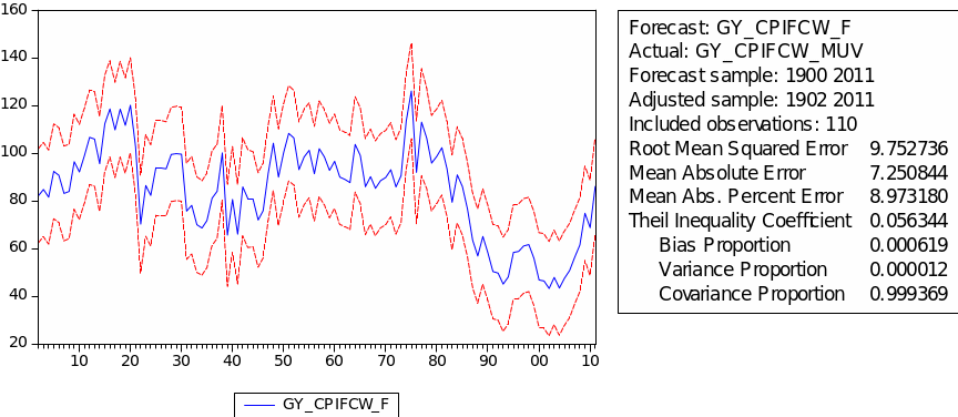
The Q-stat values suggest that these models are free from neglected serial correlation and therefore can be used to produce potentially valid forecasts for the various series.

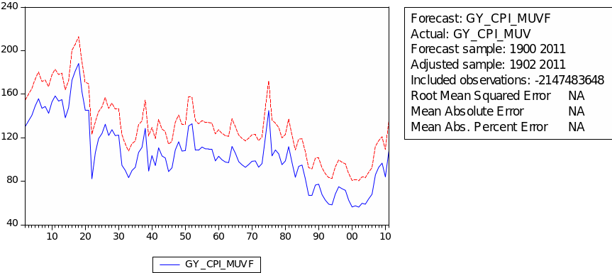
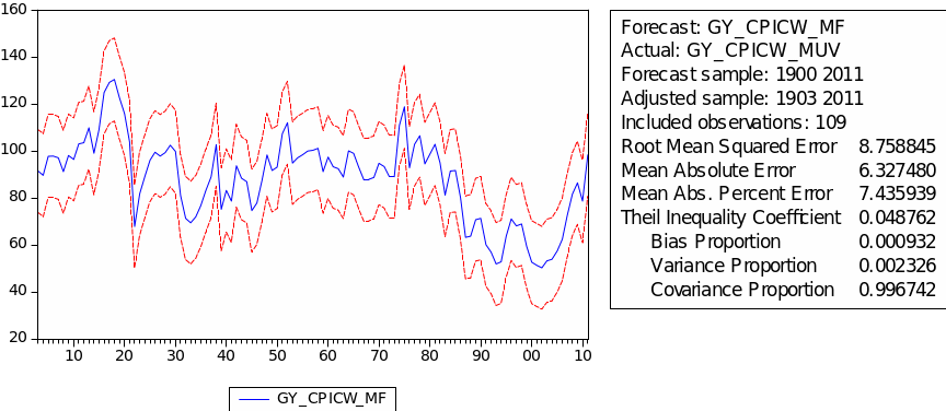
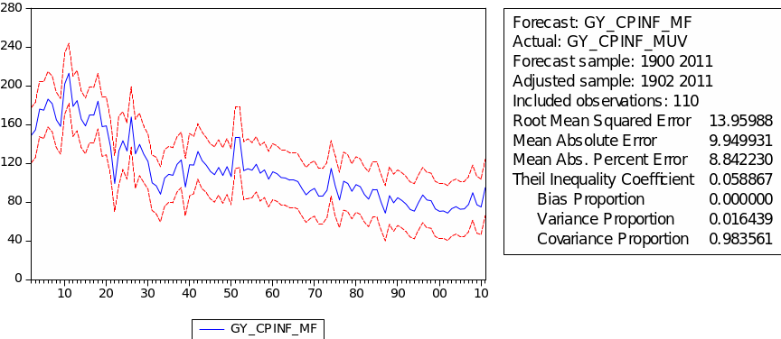
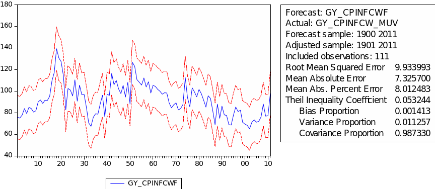
The forecast of commodity price index

The result of static forecast for every commodity price index is given is figures 1 to 8. From the result, it is easy to find that the forecast interval of geometric weights is lower than the forecast interval of arithmetic weights for each kind of index. It means that using geometric weights will make the data easier to forecast. However, we found in the literature that the decline in the relative prices of primary commodities cannot be ascertained because of the lack of long-term factor productivity growth in developing countries, the source of agricultural and mining products. Productivity growth impacts on real export prices (Grilli & Yang 1988, p. 35).

Conclusion

The research is based on examining the long-term trends of commodity price indexes. This study investigates the stationary property of each commodity price index. The period of the sample is from 1900 to 2011and includes four kinds of commodity price indexes with respect to two different weights algorithms. This study reviewed the theories and empirical studies of the various economists’ arguments on the long-term movements of commodity prices, especially on the declining trend of nonfuel commodity prices from 1900 to 2011.

In a bid to reach the main objective, many statistical methods were applied. First, augmented Dickey–Fuller test was chosen to be the method to test the stationarity of the data. There are several reasons that ADF is our choice. One reason is that this test is used by Eviews which is the statistic software chosen in this project. Stationary testing uses arithmetic weights that can ‘bring’ more stationarity.

After unit root testing, EViews was again used to complete the estimation. For those indexes with stationary property, ARMA was used for regression and for those indexes without stationary property, ARIMA was implied. To determine the lag lengths of ARMA and ARIMA models, Akaike information criterion was used.

Through the estimation of ARMA and ARIMA models, we managed to get several regression models for commodity price indexes. The Q-stat values suggest that these models can do the forecast for future values. The results presented in this thesis are important because we found that empirical evidence on the prices of exported and imported goods, particularly nonfuel primary commodity prices between developed and developing countries needs to be presented and strengthened. This was presented in the literature review and strengthened in the methodology. This study provided a glimpse of the economies of the past through prices of primary commodities and how economists relate prices with economic policies.

References

Akaike, H 1974, ‘A new look at the statistical identification model’, IEEE Trans. Auto Control, vol. 19, no. 1, pp. 716-723.

Beveridge, S & Nelson, C 1981, ‘A new approach to decomposition of economic time series into permanent and transitory components with particular attention to measurement of the ‘business cycle’, Journal of Monetary Economic, vol. 7, no. 1, pp. 151-174.

Bloomberg, S, Brock, E & Harris, E. 1995, ‘The commodity consumer prices connection: fact or fable?’, Federal Reserve Bank of New York Economic Policy Review, vol. 1, no. 3, pp. 21– 38.

Box, G, Jenkins, G, Reinsel, G 1994, Time series analysis: forecasting and control, third edn, Prentice-Hall, New York, USA.

Brockwell, P & Davis, R 2009, Time series: theory and methods, 2nd edn, Springer, New York, USA.

Cashin, P & McDermott, C 2002, ‘The long-run behavior of commodity prices: small trends and big variability’, IMF Staff Papers, vol. 49, no. 2, pp. 175-199.

Cuddington, J T 1990, ‘Long-run trends in 26 primary commodity prices: a disaggregated look at the Prebisch-Singer hypothesis’, Journal of Development Economics, vol. 1, no.1, pp. 3-18.

Cuddington, J & Urzúa, C 1999, ‘Trends and cycles in the net barter terms of trade: a new approach’, The Economic Journal, vol. 99, no. 1, pp. 426-442.

Deaton, A 1999, ‘Commodity prices and growth in Africa’, Journal of Economic Perspectives, vol. 13, no. 1, pp. 23-40.

Dickey, D, Bell, W & Miller, R 1986, ‘Unit roots in time series models: tests and implications’, American Statistician, vol. 31, no. 1, pp. 12-26.

Diebold, F & Kilian, L 1999, ‘Unit root tests are useful for selecting forecasting models. NBER Working Paper no. 6928, vol. 1, no. 2, pp. 3-28.

Garner, C 1995, ‘How useful are leading indicators of inflation?” Federal Reserve Bank of Kansas City Economic Review (2nd Quarter), vol. 1, no. 1, pp. 5–18.

Greene, W 1997, Econometric analysis, 3rd edn, Macmillan Publishing Company, USA.

Grilli, E & Yang, M 1988, ‘Primary commodity prices, manufactured goods prices, and terms of trade of developing countries: what the long run shows’, World Bank Economic Review, vol. 2, no. 1, pp. 1-48.

Gweke, J & Meese, R 1981, ‘Estimating regression models of finite but unknown order’, International Economic Review, vol. 22, no. 1, pp. 55-70.

Hannan, E 1970, Multiple time series, John Wiley and Sons, New York.

Hannan, E 1982, ‘Testing for autocorrelation and Akaike’s criterion,’ in Gani, W & Hannan, E (eds), Essays in statistical science, Applied Probability Trust, Shefield, pp. 403-412.

Hannan, E & Deistler, M 1988, Statistical theory of linear systems, John Wiley and Sons, Inc., New York.

Harvey, A 1985, ‘Trends and cycles in macroeconomic times series’, Journal of Business and Economic Statistics, vol. 3, no. 1, pp. 216-227.

Harvey, D, Kellard, N, Madsen, J & Wohar, M 2010, ‘The Prebisch-Singer hypothesis: four centuries of evidence’, Review of Economics and Statistics, vol. 92, no. 2, pp. 367-377.

Lutz, M 1999, ‘Commodity terms of trade and individual countries’ net barter terms of trade: is there an empirical relationship?’, Journal of International Development, vol. 11, pp. 859-870.

Nelson, C R & Kang, H 1984, ‘Pitfalls in the use of time as an explanatory variable in regression’, Journal of Business and Economic Statistics, vol. 2, pp. 73-82.

Perron, P 1988, ‘Trend and random walks in macroeconomic time series, further evidence from a new approach’, Journal of Economic Dynamics and Control, vol. 12, pp. 297-332.

Pfaffenzeller, S, Newbold, P, & Rayner, A, ‘A Short note on updating the Grilli and Yang commodity price index’, The World Bank Economic Review, vol. 21, No. 1, pp. 151–163.

Plosser, C & Schwert, G 1978, Money, income, and sunspots: measuring economic relationships and the effects of differencing’, Journal of Monetary Economic, vol. 4, no. 1, pp. 637-660.

Prebisch, R 1950, The economic development of Latin America and its principal problems, United Nations Economic Commission for Latin America, Michigan.

Said, S & Dickey, D 1984, Testing for unit roots in autoregressive moving-average Models with unknown order, Biometrika, New York, USA.

Sapsford, D 1985, ‘The Statistical debate on the net barter terms of trade between primary commodities and manufactures: a comment and some additional evidence’, Economic Journal, vol. 95, no. 1, pp. 781-788.

Schwarz, G 1978, ‘Estimating the dimension of a model’, Ann Statist., vol., no. l6, pp. 461-464.

Shibata, R 1976, ‘Selection of the order of an autoregressive model by Akaike’s information criterion’, Biometrika, vol. 63, pp. 117-126.

Singer, H 1950, ‘The distribution of giants between investing and borrowing Countries’, American Economic Review, vol. 1, pp. 473-485.

Spraos, J 1980, ‘The statistical debate on the net barter terms of trade between primary commodities and manufactures’, Economic Journal, vol. 1, pp. 107-128.

Thirlwall, A P & Bergevin, J 1985, ‘Trends, cycles, and asymmetries in the terms of trade of primary commodities from developed and less developed countries’, World Development, vol. 13, pp. 805-817.

United Nations 1949, Relative prices of exports and imports of under-developed countries, Lake Success, New York.

Urzúa, C M 1989, ‘Trends and cycles in the net barter terms of trade: a new approach’, Economic Journal, vol. 1, no. 1, pp. 426-442.

Von Hagen, J 1989, ‘The relative commodity prices and co-integration’, Journal of Business and Economic Statistics, vol. 1, pp. 497-503.

Whittle, P 1951, Hypothesis testing in time series analysis, Almquist and Wicksell, New York.

Whittle, P 1963, Prediction and Regulation, English Universities Press, London.

Whittle, P 1983, Prediction and regulation by linear least-square methods, University of Minnesota Press, Minnesota.

Appendix 1

The following are data and tables taken from the Grilli and Yang (1988) indexes, and shown with their 1977-1999 averages. The acronyms have corresponding data information, as explained in the literature; in particular, the CYCPIM represents the metals index; the CYCPINP for the non-food products; and the CYCPIF for the agricultural food products.

=========================== Table 1 ===========================

Table 2. GYCPI/MUV.

Table 3. The Difference of GYCPI/MUV.

Table 4. AICs for different p and q of D (GYCPI/MUV).

Table 5. ARIMA model for GYCPI/MUV.

Table 6. GYCPICW/MUV.

Table 7. The Difference of GYCPICW/MUV.

Table 8. AICs for different p and q of D (D(GYCPICW/MUV).

Table 9. ARIMA model for GYCPICW/MUV.

Table 10. GYCPIM/MUV.

Table 11. The Difference of GYCPIM/MUV.

Table 12. AICs for different p and q of D (D (GYCPIM/MUV)).

Table 13. ARIMA model for GYCPIM/MUV.

Table 14. GYCPIMCW/MUV.

Table 15. The Difference of GYCPIMCW/MUV.

Table 16. AICs for different p and q of D (D(GYCPIMCW/MUV)).

Table 17. ARIMA model for GYCPIMCW/MUV.

Table 18. GYCPINF/MUV.

Table 19. AICs for different p and q of GYCPINF/MUV.

Table 20. ARMA model for GYCPINF/MUV.

Table 21. GYCPINFCW/MUV.

Table 22. AICs for different p and q of GYCPINFCW/MUV.

Table 23. ARMA model for GYCPINFCW/MUV.

Table 24. GYCPIF/MUV.

Table 25. AICs for different p and q of GYCPIF/MUV.

Table 26. ARMA model for GYCPIF/MUV.

Table 27. GYCPIFCW/MUV.

Table 28. The Difference of GYCPIFCW/MUV.

Table 29. AICs for different p and q of D (D(GYCPIFCW/MUV)).

Table 30. ARIMA model for GYCPIFCW/MUV.

Figures 1 – 9 (Forecasts)