Statistics. Teachers’ Self-Efficacy and Gender

Introduction

This paper provides an analysis of data about the perceived self-efficacy of future teachers of mathematics. An ANCOVA will be conducted to determine whether there is a significant difference in the self-efficacy levels (the dependent variable, post_total, interval/ratio scale of measurement) between males and females (the independent variable, gender, dichotomous) while controlling for the effects of the pre-treatment levels of self-efficacy (the covariate, PRE_total, interval/ratio scale of measurement). The total sample size is N=132 (7 males, 125 females). Before conducting the analysis, the assumptions for the ANCOVA will be tested, and adjustments will be made if any of them are violated.

Testing Assumptions

Assumptions

Running an ANCOVA requires the following assumptions to be met (Field, 2013; Warner, 2103):

1. No extreme outliers in the dependent variable;
2. An approximately normal distribution of the dependent variable and the covariate;
3. A linear (and not otherwise) relationship between the covariate and the dependent variable for each level of the independent variable;
4. Homogeneity of regression slopes;
5. Homogeneity of variances for the dependent variable across groups.

Assumptions 1 and 2

The histogram in Figure 1 below shows that there are several outliers in the data for females:

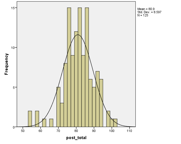
Therefore, outliers beyond 2.5 SDs (i.e., outside the interval (63.7-98.1)) will be excluded (Warner, 2013). (The mean and SD can be seen in Figure 1.) After doing this, the histogram for females becomes as shown in Figure 2 below:

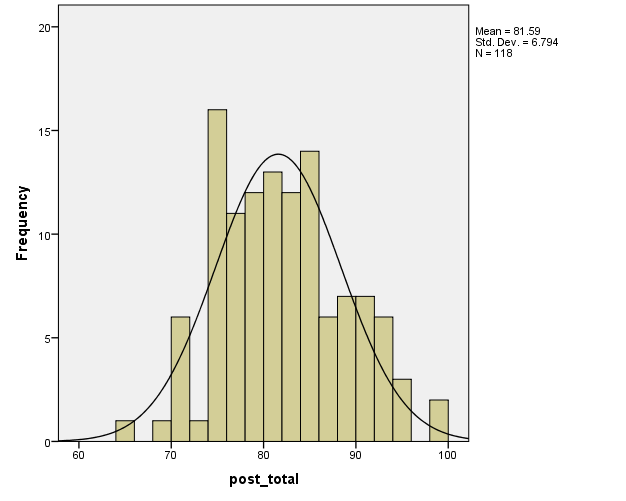
After the removal of 7 outliers, the data is apparently normally distributed for females. That the data is now approximately normally distributed for both males and females can be confirmed with the Shapiro-Wilk test (Warner, 2013), which is non-significant for both genders, which is shown in Table 1 below.

Table 1. Normality tests for post_total for different genders.

Table 2 below illustrates that the covariate is also normally distributed, for the Shapiro-Wilk test is non-significant for both males and females.

Table 2. Normality tests for PRE_total for different genders.

Assumption 3

The linearity of the relationship between the covariate and the dependent variable can be checked using a matrix of scatterplots, which is shown in Figure 3 below.

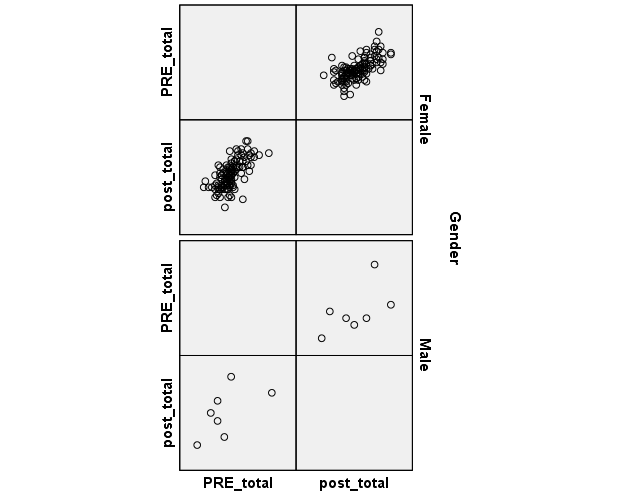
Apparently, there is no non-linear relationship between the dependent variable and the covariate on both levels of the independent variable, so the assumption is not violated.

Assumption 4

Homogeneity of regression slopes can be tested by running an ANCOVA using the custom model for the interaction between the covariate and the independent variable (the covariate and the dependent variable should also be included in the model), and examining the interaction term in the main summary table for that ANCOVA (Field, 2013, sec. 12.6). The results are shown in Table 3 below.

Table 3. Testing for homogeneity of regression slopes.

Thus, the interaction term is non-significant (p=.524), which means that the assumption of homogeneity of regression slopes has not been violated (Field, 2013).

Assumption 5

Homogeneity of variances for the dependent variable across groups can be checked using the Levene’s test of homogeneity of variances. The results are supplied in Table 4 below.

Table 4. Testing for homogeneity of variances.

It can be seen that for Levene’s test, p=.894, which means that the assumption of homogeneity of variances has not been violated.

Summary

On the whole, there were extreme outliers in the data, which have been removed (7 cases for females). No other changes in the data have been made, for it is apparent that the rest of the assumptions have not been violated.

However, it should be noted that the sample size for the males is extremely small, and, although ANCOVA is not stated to be very susceptible to different sample sizes (Field, 2013), it needs to be stressed that all the estimates for males are very approximate. In addition, there are other factors in the data which are not taken into account in the analysis, such as different courses that the respondents attended, which may further exacerbate the adverse effect of the small sample size for males.

Research Question, Hypotheses, and Alpha Level

The research question for the given analysis will be as follows: “Is there a difference in the mean scores of post-treatment self-efficacy for males and females while statistically controlling for the pre-treatment self-efficacy levels?”

The null hypothesis will state that there is no significant difference in the mean scores of post-treatment self-efficacy for males and females while statistically controlling for the pre-treatment self-efficacy levels; the alternative hypothesis will state that there is such a difference.

Because no rationale is provided for choosing the alpha level, the standard level of α=.05 will be utilized.

Results of the Analysis

The results of the ANCOVA are reported below.

Table 5. Assessment of the means for the different groups in the dependent variable.

Table 5 above shows the adjusted means of the outcome variable for different gender groups, along with the standard error and the 95% confidence intervals (the means were adjusted to the covariate). Noteworthy, the 95% CI for females is completely included in that for males. It should be emphasized that the estimates for males are much more imprecise than for females due to the small sample size.

Table 6 Results of ANCOVA.

Table 6 above provides the general results of the analysis of covariance. Evidently, Gender did not significantly affect the results of the outcome variable; F(1; 122) = 1.929, p=.167. Also, partial η²=.016, which is a small effect size (Warner, 2013); it means that approximately 1.6% of the variance in the outcome could be explained by gender.

Thus, the null hypothesis for this study cannot be rejected based on the results obtained from the used data.

Nevertheless, it can also be seen from Table 6 that the covariate PRE_total did significantly affect the outcome variable post_total: F(1; 122) = 91.283, p<.0005; partial η²=.428, which is a large effect size.

Table 7. Comparison of the means.

Table 7 displays the comparison of the means of the dependent variable adjusted to the covariate in different gender groups. Because p=.167, the difference is not statistically significant, as has been stated above.

Conclusion

Therefore, running an ANCOVA found no significant differences between the post-intervention levels of self-efficacy between males and females while controlling for pre-treatment levels of self-efficacy. However, the pre-treatment levels of self-efficacy were found to have a significant influence on the post-treatment levels of self-efficacy. A major limitation of the current analysis is the extremely small sample size of the male group of participants.

References

Field, A. (2013). Discovering statistics using IBM SPSS Statistics (4th ed.). Thousand Oaks, CA: SAGE Publications.

Warner, R. M. (2013). Applied statistics: From bivariate through multivariate techniques (2nd ed.). Thousand Oaks, CA: SAGE Publications.