When we refer to the mechanical properties of materials, whatever crosses the mind is the stress-strain curve. Ideally, both shear stress (σ) and strain (ε) testing are inevitable when it comes to material testing. While shear stress testing correlates the elongation force to the cross-sectional area of a material, tensile testing subjects a material sample to a controlled tensional force until the yield point where the material fails. The essence of performing these tests is that:
- They aid in quality control.
- Help in the selection of material meant for a specific application
- They give a glimpse of how a material would behave under varied forces.
In essence, such elements as the cross-sectional area, ultimate tensile strength as well as maximum elongation can easily be established directly. In a nutshell, from the aforementioned parameters, one is in a better position to determine the Poisons ratio, Young’s Modulus (Ε), strain-hardening, and yield strength characteristics.
Stress-strain curve diagram
A typical stress-strain diagram assumes the trend shown in figure (1) below.
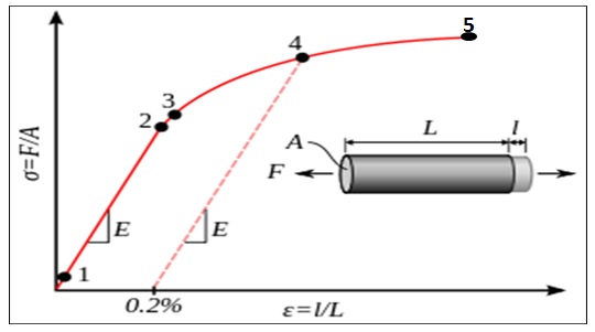
In simple terms, stress is the ratio of the elongation force to that of the cross-sectional area, while stress is the ratio of extension to that of the original length. From the graph (Fig. 1), one can obtain the Young Modulus (E) from the linear section of the curve by finding the gradient of the section (between 1 and 2).
Analyzing the graph in detail, it is important to note that point 1 is the true elastic limit, which coincides with the minimum stress that emanates from dislocations due to material movements (Egarmo et al., 2003). However, this parameter is hardly used in material science; nonetheless, it reflects a material’s chemical properties.
Between points 1 and 2, the material obeys Hook’s Law. To this end, the material stress is proportional to the deformation, and the constant of proportionality is what constitutes the Young Modulus (E). This constant is vital in the determination of a material’s stiffness. Essentially, at this point, the physical behavior of the material is such that it regains its original shape once the force is withdrawn.
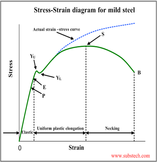
Between points 2 and 3 the material experiences elastic deformation. This point constitutes the yield limit that can elaborately be explained in figure 2 below. By definition, this is the point where an increase in stress causes a significant change in the shape of a material, deforming it. This point is defined by two points: the highest stress point YU and the lowest stress point YL (see figure 2 below). Nonetheless, the important parameter used by material scientists is the lowest stress point. Vitally, on reaching the yield limit and beyond, the material deforms permanently even when the force is withdrawn.
Finally, beyond point 3 (Fig. 1), the material is described as plastic since it has undergone permanent deformation, and it raptures at point 5. It is worth noting that there are some other materials that have an unspecified yield limit. As such, offset yield strength (point 4) at 0.2% of the origin is plotted for the sake of material comparisons.
Stress-strain diagram as used in material characterization
The essence of a stress-strain curve diagram is that it helps in material characterization. Different materials exhibit different behaviors when subjected to stress. Vitally, the physical properties exhibited by material are a manifestation of the chemical composition and the ensuing processes (thermal) that eventuates in the formation of a final product. Basically, the ensuing thermal processes determine a sample’s micro-structure and hence its physical properties. To this end, we have ductile and malleable materials. These materials can be illustrated by the curves shown in the diagram below.
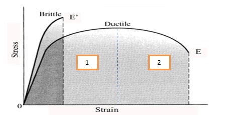
From the figure above, the difference between the two curves is visible. On the ductile trend, the curve has two sections, 1 and 2. Sections 1 and 2 represent strain hardening and the necking region, respectively. It is significant to note that the y-axis of the stress-strain graph represents the strength properties while the x-axis represents the ductility properties. Their respective behaviors are owed to the fact that brittle materials do not undergo strain hardening, consequently breaking without notice. Some examples of materials that are considered ductile include steel and copper. These are the materials that can easily be drawn into wires or worked on to obtain sheets. On the other hand, the materials that are considered brittle include concrete and glass. These materials break abruptly when subjected to stress beyond the yield point.
From the graph above, the areas under the curves illustrate materials’ toughness. Ideally, a tough material would not succumb to stress to break easily. As such, brittle materials are less tough than ductile materials. It is important to note that there are other parameters that influence the toughness of a material, which include the strain rate, temperature, the texture of the material, and the strength-ductile relationship.
How the chemical composition affects the stress-strain curve
The chemical properties of a material affect its physical properties. For instant, when we narrow down to steel as material under investigation, manufacturers alter the carbon content in order to achieve specific characteristics. For instance, with an increased carbon concentration, steel becomes less ductile, hard and stronger, and reduces welding ability. Nevertheless, the melting point decreases. Low and mild carbon steel represent steel with the lowest carbon concentrations and the most commonly used in the market. Basically, for these types, the carbon concentration is less than 0.6%. Specifically, low carbon steel (A36) has a carbon concentration of approximately 0.05-0.3%, while the mild carbon steel (1040) exhibits a concentration of roughly 0.3-0.6%. As a consequence, this enhances the metal’s malleability and ductility characteristics. With a carbon content of approximately 0.6-0.99% (4140), high carbon steel exhibits relatively high strengths; thus, it finds application in springs. On the other hand, ultra-high carbon steel (1-2% carbon content) exhibits unprecedented hardness vital in making axels and knives (Day, 1998).
The illustration above of the stress-strain diagram underscores the need for one to understand the behaviors of different materials under varying stress. As demonstrated in the diagrams above, this knowledge is vital in the quality control, selection of a material meant for a specific application and gives a glimpse of how a material would behave under varied forces. With these illustrations, it is important to note that ductile materials are relatively tougher than brittle materials and hence can withstand excessive stress without failure. These materials would be best applied, where excessive force is needed.
References
Day, J. (1998). The Bristol Brass Industry: Furnaces and their associated remains. Journal of Historical Metallurgy, 22, 19-24.
Egarmo, E., Black, J., & Kohser, A. (2003). Materials and Processes in Manufacturing (9th ed.). New York: John Wiley & Sons.
Groover, P. (2007). Fundamentals of Modern Manufacturing: Materials, Processes and Systems (3rd ed). New York: John Wiley & Sons.